

Introduction
Mozambican Common Beans Market
Materials and Methods
Data
Descriptive Statistics
Model Selection
Optimal Lag Selection
Stationarity Test
Co-Integration Test
Testing for Granger Causality
Testing for Asymmetry
Results
Optimal Lag Selection Criteria
Stationarity Test
Co-integration Test
Modeling Short-run Causality in the ARDL Model
Testing for Long-run Causality in the EC Model
Discussion
Introduction
Many contemporary economics practitioners have been drawing their attention on analyzing price relationships across spatially separated markets, especially for the main and emergent agricultural commodities which are relevant not only by the economic point of view – as a source of income, but also in the social angle, since they are consistently the staple food.
In Mozambique, the common beans are one of the most produced, consumed, and commercialized commodities (Chaves, 2011). The Agriculture and Food Organization of the United Nations (FAO) statistics show that the total production reached roughly 51,000 tons in 2018 (FAOSTAT, 2018), what reveal the magnitude of importance that this commodity assumes for the country. The Human Development Report from the United Nations Development Programme (UNDP, 2019) cite Mozambique as one of the countries with the lowest index of human development. Most of the population live in the rural area (INE, 2018) with unstable livelihood means. Abbas (2017) argues that the availability of basic food commodities in Mozambique, including common bean, is very low. This can be also linked to the high rates of post-harvest losses, derived from poor conditions of storage, and lack access to markets.
The agricultural markets in Mozambique are divided in three main segments, to be more specific, farm, wholesale, and retail levels. The Annual Agricultural Statistics (2018) reports denote that the higher amount of the national gross production in common beans come from the central and northern regions. In general, the flow of beans along the supply chain is north-south with an involvement of many informal traders (SIMA, 2019). The degree of market integration is a major determinant in promoting the well-being of consumers, including the sharing of benefits among the players within the transactional market and has a great influence on food security, especially in developing countries, such as Mozambique, where most of the population have a lower purchasing power. Ozgur et al. (2014) state that tremendous difference between farm gate and retail prices cannot be only related to cost and other factors, but perchance by the existence of considerable market power which can result from non-competitive markets.
The existence of market power is one of the main sources of possible asymmetries and, according to Balke and Goshray (1997), it may be evidence that the producers are using their market force, or the that the retailers are benefiting from the last users’ search costs. The transactions along the common beans markets take place in an environment mainly characterized by precarious roads, long distance between the farming areas and main consumer centers, lack access to market information, including some localized focus of military conflicts, what foreclose the movement of people and goods, therefore it becomes relevant to assess the market integration and price transmission among the farm, wholesale, and retail markets of common beans in Mozambique. The main purpose of this study is to analyze the market integration and price transmission along the common beans supply chain in Mozambique and the specific objectives are (i) to analyze the spatial price relationship among farm, wholesale, and retail markets of common beans in Mozambique, (ii) to identify the price leadership among the farm, wholesale, and retail markets of common beans, and (iii) to analyze the speed of adjustment on shocks in the long-run equilibrium of the common beans market. Finally, we examine the existence of asymmetric response on shocks to the common beans market in Mozambique.
Assessing for market integration and price transmission is substantially crucial since it provides a discernment to determine whether there is a need of government intervention to reduce or correct the market inefficiencies, especially for the main commodities which are the source of family subsistence and they have an important role on the food safety, such as common beans in Mozambique. Likewise, there are few studies related to this topic for agricultural commodities in Mozambique, except the study undertaken by Chaves (2011), addressing the issue of market integration, however, his study was only based on analyzing the integration between the wholesale markets. In this study, we extend our analysis to the entire common beans supply chain, playing a contribute to cover the gap on information related to this topic.
Previous studies have examined market integration and price transmission across marketing channels in agricultural commodity markets (e.g., Abdulai, 2000; Aguiar and Santana, 2002; Capps and Sherwell, 2007; McLaren, 2015, etc.). Their results are heterogenous across different regions and products. This study contributes on related literature by adding the case of Mozambique, which is relatively lower income country in Africa.
Mozambican Common Beans Market
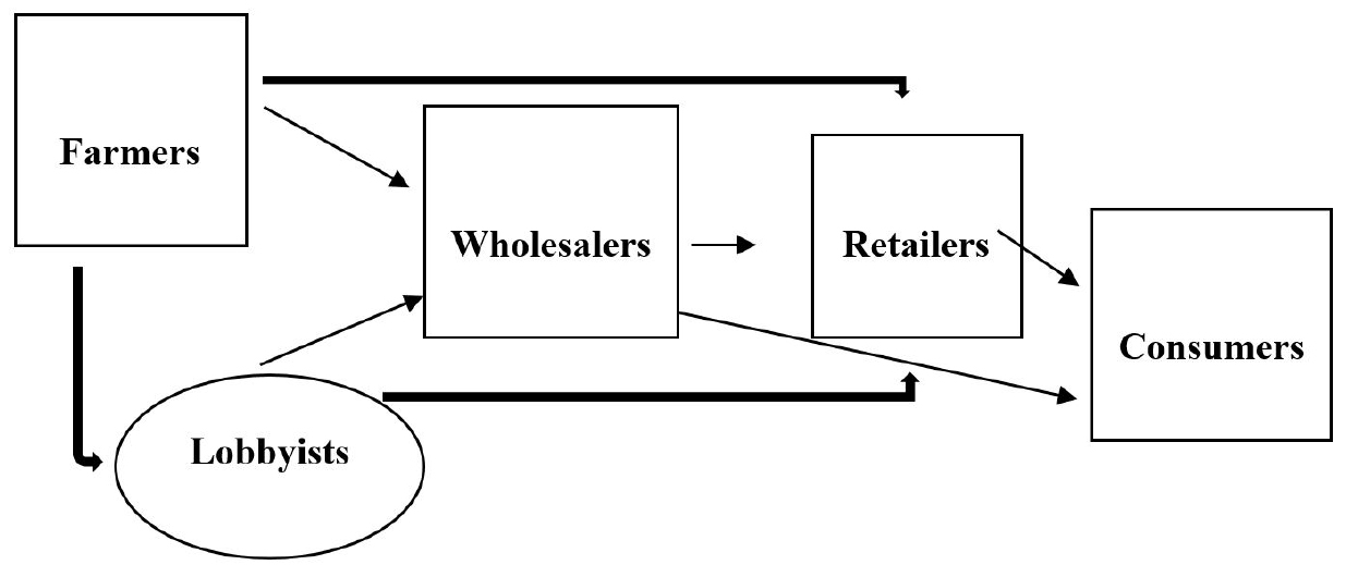
Mozambique is located at the Eastern cost of the Southern Africa region, and has 11 provinces split into three regions, namely South, Central and Northern. The Central and Northern regions contribute with the larger amount on the national gross agricultural production, including common beans (Annual Agricultural Statistics, 2018). The common beans market structure is composed by farmers, lobbyists, wholesalers, retailers, and consumers. The informal relationship between these stakeholders is described in Fig. 1 below. Common beans farmers sell their product to the wholesalers and retailers with or without lobbyists intervention, and in some occasions, farmers are also part of the wholesale market structure. Retailers are the ones who have linkage with the last consumers and they obtain the product either from the wholesalers or farmers, however some consumers also purchase the product from wholesalers. Lobbyists are usually people living in the farming areas who are related to the downstream markets (wholesale and retail). They play a role on trading information to the wholesalers and retailers about the location and prices at the farm gate and in most of the occasions they are responsible by organizing the farmers on the sale day or collecting the common beans from the farmers in the sense that the wholesalers and retailers can avoid addressing the issue of geographical dispersion of farmers. This role allows them to gain economic benefits either from farmers or wholesalers and retailers.
The common beans market flow is north-south (SIMA, 2019), since the highest production comes from the northern and central regions and the biggest consumer centers are located in urban areas of the southern region to attend the demand which is increasingly high due to migration of the population from the rural areas to the towns. Has an underdeveloped country, Mozambique has poor road conditions and lack of communication means what contributes to weaken the linkage between the farming areas and the consumer centers. The high transportation costs are associated to the long distance from the farming zones to the urban areas, with impact on the last price that the consumers are supposed to pay and it can lessen their purchase power which is already weak, affecting the food security of lower income households that have the common beans as their main source of proteins. It is also important to mention that some potential and localized armed conflicts also constitute a barrier to the linkage between farming areas and consumer markets.
Markets are considered to be performing efficiently if the price signs (changes) are completely transmitted along the different levels. The main requirement for market efficiency is that all the available information has to be incorporated and be reflected on the actual market prices. Once the availability of market information increases, the markets will simultaneously increase their efficiency, leading to the elimination of arbitrage. The factors mentioned before are catalytic for the market inefficiency, so it becomes relevant to assess the spatial price transmission and asymmetry in the common beans market, to provide a clue about policy direction to target the main sources of market inefficiency, since there are few studies related to this topic, other than the one from Chaves (2011), which only focused on analyzing the integration between the wholesale markets of common beans in Mozambique.
Materials and Methods
Data
Since the aim of this study is to evaluate the short- and long-run asymmetric price transmission and co-integration along the common beans supply chain in Mozambique, secondary data is used which consists of price series of three main channels, namely farmer price (lnfpr), wholesale price (lnwpr), and retail price (lnrpr). In total, 137 observations from 2017 to 2019 for each variable are used, and this period was chosen based on the consistence of the data available from the data source. All the series consist of weekly average farm, wholesale, and retail prices, consistently recorded during the period in allusion, allowing to stablish the price relationship along the whole common beans supply chain.
All the prices were obtained from Quente-Quente which is the weekly bulletin of the Agricultural Market Information System (SIMA) of the Ministry of Agriculture and Rural Development of Mozambique, the official entity responsible on collecting, analyzing, and keeping all the statistics related to agricultural markets in the country. All the prices were previously converted into natural log form before performing the proposed analysis.
Descriptive Statistics
Providing the summary statistics is one of the key-steps on pursuing quantitative analyses since it can provide a very useful information about the main characteristics of the data we are dealing with, allowing us to select the appropriated method when we proceed to in-depth analysis. The Table 1 below shows the descriptive statistics for the three price series. The variables are described as farm price (fpr), wholesale price (wpr) and retail price (rpr) and all the prices are in Metical (MZN), the Mozambican currency.
Table 1.
Summary statistics
The farm average price is 53.16 MZN, and the minimum and maximum values observed on the farm price series are respectively 28.87 and 86.61 MZN. The standard deviation (12.43) shows that the observations on farm price are far from the average value and the variance (154.61) shows that the observations have a wide variation from the mean value. This tendency remains the same when we look at the summary statistics of the wholesale and retail price series. When we look at the skewness values we can clearly conclude that farm and retail prices have a normal skewness, while the wholesale price has a long-right tail (positive skewness). The Kurtosis values show that among the three price series, only the wholesale price is normally distributed.
Model Selection
Empirical exercises to test the predictions obtained from economic theory are largely used on scrutinizing price transmission, however it’s important to mention that they can mostly be explained using the point-location model (Fackler and Goodwin, 2001), that expresses the equilibrium condition in the Law of One Price. Most of the early studies on price transmission have been censured since they were only applying correlation test and simple regression analyses, ignoring the nonstationary proprieties of price time series data (Barrett, 1996). This suggest that there are bunch of time series techniques that must be used to address the nonstationary nature of price data in order to avoid pursuing spurious analyses.
In our study, we use the Autoregressive Distributed Lag (ARDL) model by Pesaran et al. (2001). We choose this model since it comports many advantages since it can be used to analyze the relationship between series of different order of co-integration, i.e., I(0) and I(1), it also includes a test on co-integration and an error correction model, allowing to capture both short-run and long-run relationship. Afterwards, we proceed using the nonlinear ARDL model (Shin et al., 2014) to capture the asymmetry by modeling the effect of positive and negative changes on the impulse variables.
Optimal Lag Selection
The economic theory can be used as one of the vade-mecum for optimal lag selection, given a prior information about the nature of specific economic variables, however, the optimal lag determination is not only limited to that. There is also a series of statistical methods that can be used to determine the optimal lag order, such as the Akaike Info Criteria (AIC), Bayesian Information Criterion (SBIC) and Hannan-Quinn Info Criteria (HQIC). For that purpose, our study uses the AIC and SBIC (Hamilton, 1994), which can be expressed by the following equations:
where SSR is the sum of the residual squares; T is the length of the sample (number of observations); p is the lag length that minimizes the respective criterion (AIC).
Stationarity Test
As highly recommended by many scholars (McNew and Fackler, 1997; Fackler and Goodwin, 2001; Barrett, 1996), the first step undertaken in this study is to check whether the time series contains unit roots or not using the Augmented Dickey-Fuller (ADF) procedure (Dickey and Fuller, 1979). As the visual inspection of the data plots (recommended by Gujarati and Porter, 2009) suggest the existence of unit root, the ADF test is performed including a trend, in the sense that the constant is allowed to be unrestricted, to test the null hypothesis that the variables have a unit root, following the equation below:
where are the individual price series and is the pure white noise error term that follow a normal distribution with zero mean and is the number of lags included in the model do allow the white noise term to have zero mean and constant variance.
The lags length used in the ADF test is chosen based on the Akaike Information Criterion (AIC) and Bayesian Information Criterion (SBIC). The ADF test involves fitting the regression model using ordinary least squares (OLS), allowing for higher-order autoregressive process by including in the model to attend for serial correlation problems.
Co-Integration Test
After addressing the issue of data stationarity and confirming that the series are integrated at the same order, the following step on estimating the price transmission is pursuing the co-integration test (Engle and Granger, 1987; Johansen, 1988). This will lead to a better choice of the model that best fits the data, considering the number of variables and vectors. For that purpose, this study explores the autoregressive distributed lag (ARDL) procedure developed by Pesaran and Shin (1995) and Pesaran et al. (2001), since it has advantages if compared to other traditional methods as postulated by Harris and Sollis (2003), because even though the series are not integrated at the same order, i.e., I(0) and I(1), it still provides efficiency when it is applied in the analysis of long-run relationships and short-run dynamics. The bounds test is performed in two steps. The first step is to estimate the long-run relationship between the price series. If the series are co-integrated, it implies that they are related and can be combined in a linear fashion, meaning that even if there are shocks in the short-run, which may affect the movement in the individual series, they would move to converge in the long-run equilibrium, and consecutively, the second step is to estimate the short-run relationship. The bounds test is based on the following generalized ARDL equation:
where is the vector and the variables in are allowed to be purely I(0) or I(1) or co-integrated; and are coefficients; p and q are the optimal lag orders; is a vector of error terms – unobservable zero mean white noise vector process (serially uncorrelated or independent).
As this study uses the bounds test to inspect the relationship between three variables (retail, wholesale and farmer prices – all in log form), the bounds test for co-integration using the conditional ARDL is specified as:
where lnrpr, lnwpr and lnfpr are respectively the retail, wholesale, and farmer prices in their log forms, and eit is the white noise term for each bound.
Testing for Granger Causality
Has we described before, the ARDL model also captures the short-run and long run relationship between the variables. Thus, after performing the bounds co-integration test, we proceed testing for short-run and long-run granger-causality where the series are proved to be co-integrated and we test only for short-run granger-causality where it is found no co-integration, following the equations (8), (9) and (10) below:
where is the speed of adjustment; ECT = (Response variablet-1-θXt) is the error correction term which is extracted from the residuals of the regression (note that the equation (8) does not include the ECT since when the wholesale price is treated as exogenous, it was not found co-integration, thus we only estimate the short-run model); is the long-run parameter; and a1i, a2i, a3i are the short-run dynamic coefficients.
Testing for Asymmetry
The results of the granger-causality test give a clue about the way-forward on modeling the relationship between the price series. If price leadership is identified between the market pairs, the following step is to test for asymmetry. For that, we employ the nonlinear ARDL developed by Shin et al. (2014) to obtain the short-run and long-run dynamic multipliers, expressed in the following general equation:
where and are the asymmetric distributed lag parameters, and are the associated asymmetric long-run parameters. The nonlinear ARDL model developed by Shin et al. (2014) is considered as an extension of linear ARDL model. The main difference between linear ARDL and nonlinear ARDL is that nonlinear ARDL model does not assume symmetric impacts of x on y. Therefore, nonlinear ARDL model can capture the potential asymmetric effects.
Results
Optimal Lag Selection Criteria
Before pursuing formal analysis using the models, it is advisable to determine the lag length which is suitable for the variables, either taken individually or cluster, in the sense that we avoid inflations on standard errors of coefficient estimates or incur to a bias estimation, due to wrong lag specification. Table 2 show the results of lag selection criterion, that lead us to choose the optimal lag length based on the Akaike Info Criteria (AIC) and Bayesian Information Criterion (SBIC).
Table 2.
Optimal lag selection criterion
| Lags | df | P | AIC | HQIC |
| 0 | - | - | -2.07954 | -2.05305 |
| 1 | 9 | 0.000 | -5.875921) | -5.769941) |
| 2 | 9 | 0.730 | -5.78641 | -5.60096 |
| 3 | 9 | 0.768 | -5.69401 | -5.42908 |
| 4 | 9 | 0.801 | -5.59905 | -5.25464 |
Stationarity Test
The ADF test results (Table 3) show that only the farmer price series are stationary at the level. It can also be noted that the retail price series show to be stationary when the trend term is not included, however when we include the trend term, they do not remain stationary. Although all the price series become stationary when their first difference is taken, since they maintain the stationarity condition, no matter if a trend term is included or not, this imply that we are in presence of series of different order of co-integration. The lag length for the ADF test was decided following AIC and SBIC.
Table 3.
ADF test
| Variables | t-statistic | Critical value | Decision | ||
| Trend | No trend | Trend | No trend | ||
| lnrpr | -3.181 | -3.087 | -3.445 | -2.888** | Non-stationary |
| lnwpr | -2.471 | -2.290 | -3.445 | -2.888 | Non-stationary |
| lnfpr | -4.019 | -4.084 | -3.445** | -2.888** | Stationary |
| Δlnrpr | -12.240 | -12.177 | -3.445*** | -2.888*** | Stationary |
| Δlnwpr | -12.906 | -12.312 | -3.445*** | -2.888*** | Stationary |
| Δlnfpr | -8.255 | -8.137 | -3.446*** | -2.888*** | Stationary |
Co-integration Test
Testing for co-integration is one of the preliminary issues when we are modeling the relationship between price series, since it allows us to determine the number of co-integrating vectors for the set of data series. For that, we use bounds co-integration test which is performed in three steps, since our study uses three variables, where in each step, we commute the variables allowing them to be treated as exogenous to test for co-integration using the AIC for the optimal lag selection. Table 4 shows the results of co-integration test and based on them we can see that when the farm and retail prices are treated as exogenous variables, there are at least two co-integrating vectors between the farm, wholesale and retail prices. However, when the wholesale price is considered as the outcome variable, the results show no co-integration. This is an evidence that three prices will move to converge in the long-run even if shocks in the short-run may induce them to a different tendency.
Table 4.
Bounds co-integration test results
| Response variable | Tests | Critical Bounds | Decision | |
| I_0 | I_1 | |||
| lnfpr | F-statistic 10.965*** | 5.15 | 6.36 | co-integration |
| t-statistic -5.651*** | -3.43 | -4.10 | ||
| lnwpr | F-statistic 2.613 | 5.15 | 6.36 | No co-integration |
| t-statistic -1.908 | -3.43 | -4.10 | ||
| lnrpr | F-statistic 6.740*** | 5.15 | 6.36 | co-integration |
| t-statistic -4.188*** | -3.43 | -4.10 | ||
From the explanations of the previous results, it is clear that although some of the analysis can give us an idea about the long-run relationship between the retail, wholesale and farm prices of common beans, none of them could be taken as conclusive to infer about the long-run. Accordingly, we proceed testing for granger-causality using ARDL model. For that, we perform the ADRL test in three steps, as we conducted on the co-integration test. The previous results on bounds test suggest how granger-causality have to be addressed, thus we will proceed testing for granger-causality using the simple ARDL where was found no co-integration and error correction model (ECM) where is proved that there is co-integration.
Modeling Short-run Causality in the ARDL Model
As we stated before, the evidence of no co-integration clearly indicates that on that particular direction there is no long-run relationship between the variables. Therefore, we proceed testing for short-run relationship among the price series using the simple ARDL model. The same procedure is applicable for the co-integrated vectors, since it is also important to diagnose the short-run relationship between the variables.
The results are displayed on Table 5 below, and their interpretation allows us to say that in the short-run, the wholesale price has a significant effect to its own changes when it is taken as response variable, with a positive coefficient at the 1% level of significance. It is also notable that the retail price has a negative effect on the wholesale price in the short-run at the 10% significance level, however the farm price does not show a significant effect on the wholesale price. All the interpretation of the ARDL results is subject to ceteris paribus assumption.
Table 5.
Short-run Granger causality by ARDL model
| Dependent variable | Independent variable | coefficient | t-statistics | P-value |
| lnwpr | Lnwpr (-1) | 0.9369*** | 28.34 | 0.000 |
| Lnfpr (-1) | 0.0329 | 1.21 | 0.229 | |
| Lnrpr (-1) | -0.0570* | -1.67 | 0.098 | |
| Const. | 0.3772 | 2.52 | 0.013 | |
| lnrpr | Lnrpr (-1) | 0.8113*** | 18.02 | 0.000 |
| Lnwpr (-1) | 0.0383 | 0.85 | 0.395 | |
| Lnfpr (-1) | 0.0815** | 2.20 | 0.029 | |
| Const. | 0.3527 | 1.64 | 0.104 | |
| lnfpr | Lnfpr (-1) | 0.5914*** | 8.18 | 0.000 |
| Lnwpr (-1) | 0.2483*** | 2.96 | 0.004 | |
| Lnrpr (-1) | 0.1377 | 1.52 | 0.130 | |
| Const. | -0.0051 | -0.01 | 0.990 |
When the retail price is considered as the outcome variable, it is noticed that it has a positive significant response to own changes at the 1% significance level and the farm price also shows a positive effect on retail price at the 5% significance level. However, we failed to reject the null hypothesis of no significant effect when we look at the wholesale price. Flipping the change to farm price as the dependent variable, we find a positive significant effect on own response and also a positive effect of the wholesale price at the 1% of significance level. The retail price shows a significant effect on the farm price, ceteris paribus.
Testing for Long-run Causality in the EC Model
Given the existence of co-integration when we treated the farm and retail prices as exogenous variables, we test for long-run granger-causality using the EC model which is an extension of the ARDL model, which apart from the short-run results of the simple ARDL, provides a long-term adjustment coefficient (Table 6).
Table 6.
Long-run Granger causality by EC model
| Dependentvariable | Independent variable | Coefficient | t-statistic | P-value |
| lnrpr | lnrpr (adj.) | -0.1886*** | -4.19 | 0.000 |
| lnwpr | 0.2034 | 0.84 | 0400 | |
| lnfpr | 0.4325** | 2.27 | 0.025 | |
| lnfpr | lnfpr (adj.) | -0.4085*** | -5.65 | 0.000 |
| lnwpr | 0.6077*** | 3.30 | 0.001 | |
| lnrpr | 0.3370 | 1.66 | 0.100 |
When the retail price is taken as the outcome variable, the error correction model results show that in the long-run, the farm price has a significant effect on the retail price at the 5% significance level. A percent increase on the farm price is associated with 0.43% increase in the retail price. However, the wholesale price appears to not have a significant effect on the retail price and, as described in the market structure, this can be associated to the fact that some retailers do not rely on the wholesale market to obtain their product since they can have direct contact with the farmers to buy common beans. The EC model also shows that roughly 0.19% of the errors from the previous period will be corrected in the current period and the negative adjustment coefficient (-0.1886) shows convergence in the long-run equilibrium.
The wholesale price has a significant effect on the farm price in the long-run, when the farm price is considered exogenous variable. If there is 1% increase in the wholesale price, the farm price will respond with an increase by 0.61%. This might be a result of the farmer participation in the wholesale market structure, what allows them to have a better exploitation of the market information at this level to increase their commercial margins. The long-run adjustment coefficient explains that previous period errors are corrected in the present period in 0.41% and the negative sign shows a long-run convergence. We present the summarized granger-causality test results in the following Table 7.
Table 7.
Summary of Granger causality test results
From the Table 7, it is clear that the retail price leads the wholesale price and the farm price leads the retail price, both in the short-run and long-run, while only in the short-run the wholesale price leads the farm price. All the price leadership has a unidirectional granger-causality. The price leadership between the market pairs is a clear suggestion of the existence of price asymmetry, thus we proceed testing for short-run and long-run price asymmetry, pairing the prices in three ways, as indicated by granger-causality test results. In the following Table 8, we display the asymmetric results using a nonlinear ARDL framework (Shin et al., 2014) for both short and long-run dynamics multipliers.
Table 8.
Results of the asymmetric nonlinear ARDL Model
| Retail – Wholesale | Wholesale – Farm | Farm – Retail | ||||||||
| Coef. | t-Stat | Coef. | t-Stat | Coef. | t-Stat | |||||
| _xlp | 0.0042 | 0.08 | _xlp | 0.3234*** | 3.40 | _xlp | 0.1329*** | 3.36 | ||
| _xln | -0.011 | -0.25 | _xln | 0.3367*** | 3.34 | _xln | 0.1441*** | 3.62 | ||
| 0.055 | 0.01 | 0.777*** | 17.71 | 0.450*** | 11.2 | |||||
| 0.143 | 0.05 | -0.808*** | 17.84 | -0.489*** | 14.58 | |||||
We perform the asymmetric nonlinear ARDL using 2 lags, since this is the minimum requirement shown on the lag matrix provided by the model. The _xlp stands for response on the positive change and _xln for negative changes response, both in the short-run while in the long-run, and stand for positive and negative response, respectively. For the retail-wholesale market pair, we failed to reject the null hypothesis of no asymmetry, because the coefficients positive and negative change response do not differ significantly from zero. The coefficients of the wholesale-farm and farm-retail market pairs differ significantly from zero, both in the short-run (_xlp; _xln) and long-run (), what explains that the price series will converge in the long-run. The farm price responds differently on the wholesale price increase and decrease. Although both induce a positive change, the farm price reacts faster to the wholesale price decrease than it does to the wholesale price increase, since the wholesale price decrease induces a significant greater increase on the farm price than the wholesale increase does, both in the short-run and long-run at the 1% significance level.
This tendency remains the same when we look at the retail prince response on positive and negative changes to the farm price increase. For both market pairs, the null hypothesis of no asymmetry is rejected, when relying on the asymmetric nonlinear ARDL results, what is consistent with the results obtained by Chaves (2011), regarding to market integration and price transmission along the wholesale common beans markets in Mozambique.
Discussion
The common beans market in Mozambique is liberalized, allowing the sellers and buyers at different levels (farm, wholesale. and retail) to have a free interaction, since there is no government market intervention. Most of the producers of common beans in Mozambique are small holder’s farmers, and they are not actually doing farming as a business, but for their family subsistence, however they often get involved in the market chain since they sale their surplus in order to obtain money to fulfil other needs, such as education and health.
Many programs oriented to develop rural markets have been implemented by government and partners, as a contribution to develop the rural areas leading the small scale farmers to migrate from food farming to business oriented agricultural activity and the common beans are one of the commodities they are prone to get involved on trade, since its demand is increasingly high.
The difference between the farm price and retail price in the common beans market suggests that the transaction costs are high. The long physical distance from the farming areas to the main markets, the precarious roads and military conflicts are the main barriers to the free trade and might be one of the reasons there is a high difference between price at the farm gate and at the retail level. This suggest that there is a need of investment government policy to improve the roads conditions and safety to enable a free movement of people and goods. It could also be considered a possibility of using other means of transport, such as sea and rail transport, which are proved to be effective on reducing the costs involved on people and goods transportation.
The price asymmetry along the supply chain indicates the existence of a relative market power that can lead to market inefficiency. Farmers in rural areas are most likely to have informal groups and they usually organize themselves to sell their products in the same location and day, what allows them to have a mutual agreement about the sale price of common beans, led by the information obtained from the wholesale level, since some farmers are also part of the wholesale market structure. On the other side, the retailers who also compete with the wholesalers to buy the common beans from farmers, exercise their market power by better exploitation on the market information, what enables them to maintain or extend their profit margins. All this collusive behavior has impact on price stability of common beans in Mozambique, and it affects the food safety of low-income households, who have the common beans as the main source of proteins in their food regimen.
Most of the farmers, wholesalers, and retailers of common beans in Mozambique are in the informal sector, thus it is quite difficult for the state entities to have a total control about them, including tracking the information in terms of transactions which occur in this sector. The market informality can also be a source of market asymmetry leading to market inefficiency. This suggests that a policy is required to target the transformation of the agricultural markets into a formal sector. This transformation could also be the step forward on market specialization since, as described in the market structure, the market stakeholders play multiple roles along the supply chain, and this can also be a source of market inefficiencies.
Mozambique is integrated in the free trade region of the Southern African Development Community (SADC) meaning that the national markets are prone to receive or export agricultural products, including common beans. This brings about another challenge in terms of tracking all the information related to those transactions and also to measure their effect in the local prices, and from the information available currently, it is noticed that these transactions are not specified.
Naturally, the interpretation given to these results is restricted to common beans markets for the period analyzed, however the situation can be similar or even worse for other agricultural commodities, since the market landscape is quite similar. Therefore, further in-depth research is recommended, not only for common beans market, but for other main crops, since they can provide insights for policy delineation. In addition, given our data period restriction, the readers should be cautious about generalizing our results in common bean market.
