


Introduction
Background
Data and Methodology
Empirical Model
Results and Discussion
Own-Price Elasticities (Short-Run)
Cross-Price Elasticities (Short-Run)
Expenditure Elasticity
Application of Results to Crop Programming
Conclusion and Policy Recommendations
Introduction
Vegetable farming is colloquially equated to gambling, where farmers who are able to sell their produce at high prices are said to have hit the jackpot. Indeed, vegetables cultivation has made several farmers instantly rich, but it has also left others in previously unimagined debt. In times of a vegetable glut, it is common to see vegetables dumped along the roads or just left unharvested, which happens almost every year (Albano, 2025). For instance, Macatuno and Quitasol (2024) reported that between December 20-30, 2023, about 8 million kilograms of assorted vegetables valued at around ₱240 million remained unsold and were at the risk of dumping due to oversupply and depressed prices.
Similarly, Agoot (2025) noted that the influx of supply has often caused drastic price decline, leaving many farmers unable to recover even half of their production costs. In extreme cases, farmers have resorted to giving away or donating unsold vegetables, with some using social media to invite public to collect the produce for free. Others simply let their harvests rot due to unprofitable selling conditions. Vegetables that have experienced oversupply and/or dumping episodes include cabbage (Araneta, 2024; Cariaso, 2024; Miranda, 2020), carrot (Casucian, 2025; Meddler, 2019; Rita, 2019), tomato (Cariaso, 2023; Manahan, 2025; Untalan, 2025), potato (Ignacio, 2019), and squash (Borja, 2023; Fernandez, 2023). These recurring incidents suggest that vegetable dumping remains a recurring concern in the Philippine agriculture.
National and regional media coverage of these events has prompted calls for structural solutions. Cabrera and Wagey (2024) urged stakeholders to address the issue and suggested that one of the factors that need to be studied in this situation is supply-demand scenario since supply changes in response to market demand. Meddler (2019) identified the lack of effective crop programming as one contributing factor to the vegetable dumping. In response to these incidents, the Department of Agriculture (DA) is pushing for a cropping calendar across the country, in a bid to ensure that there is no wastage as farmers have been throwing out produce due to oversupply (Cabuenas, 2022). Notably, Agoot (2022) emphasized that data from 2017-2022 indicate that prices do not necessarily decline when supply is abundant, suggesting that demand conditions may play an important role.
At the same time, several studies have examined vegetable consumption patterns in the Philippines. Conception (2009) found that in Mindanao, most purchased vegetables include squash, eggplant, ampalaya, okra, string beans as well as tomatoes, potatoes, and cabbages with average purchase quantities ranging from 250 to 600 grams. In Isabel, Leyte, households commonly consume moringa, squash, eggplant, okra, carrots, and cabbage (Saloma, 2022). Among high school students in Cavite, squash was identified as the most preferred vegetable (Gonzales et al., 2024). Ironically, many of the vegetables identified as commonly purchased consumed are also those frequently associated with oversupply or dumping incidents.
Paradoxically, despite periodic oversupply, national data indicate that Filipinos’ fruit and vegetable intake remains below recommended levels. During the 2022 third quarter meeting of the National Banner Program Committee on High Value Crops-Fruits and Vegetables, the Food and Nutrition Research Institute (FNRI) reported that per capita consumption from the 2018-2019 Expanded National Nutrition Survey fell short of the 400 grams per day recommended by the World Health Organization (WHO). In rural Isabel, Leyte, estimated daily per capita vegetable consumption was approximately 48.28 grams (Saloma et al., 2022). These findings indicate that under-consumption coexists with recurring oversupply, suggesting inefficiencies in market coordination rather than a simple surplus of production.
Empirical demand literature on vegetables in the Philippines remains limited. Mutuc et al. (2007) noted that empirical work focusing on vegetable demand has been sparse. Most Philippine demand studies examined vegetable as an aggregated commodity, while only a few disaggregated vegetables into finer sub-categories such as green, leafy, yellow, and fruit vegetables. The commodity level empirical demand study by Mutuc et al. (2007) with an additional exploration of effects of socio-demographic factors and urban/rural dummy variables on vegetable food demand, included only two of the vegetables (cabbage and tomato) that are commonly associated with oversupply or dumping issues. To date, there remains limited evidence estimating commodity-level own-price, cross-price, and expenditure elasticities for vegetables frequently affected by glut conditions.
The objective of this study, therefore, is to examine vegetable demand behavior at a commodity level as an input for crop programming. Particular emphasis on calculating the expenditure, own and cross price elasticities of commonly dumped vegetables and has supply glut incidents in the Philippines. Specifically, the study estimates own-price, cross-price, and expenditure elasticities for vegetables that have been frequently associated with supply glut and dumping incidents in the Philippines. By linking elasticity estimates to production planning considerations, this study contributes to the limited empirical literature on disaggregated vegetable demand and provides evidence-based inputs for developing a market-oriented crop programming strategy.
The remainder of the paper is organized as follows: section 2 presents the background and conceptual framework. Section 3 describes the variables, and econometric methods used. Section 4 discusses the empirical results, Section 5 concludes with policy implications and recommendations, and Section 6 is the appendix.
Background
Crop programming refers to the systematic planning and coordination of vegetable production based on many factors such as land and soil, water resources, inputs, labor and machinery, market access (price and demand), and risk management considerations. Traditionally, vegetable production decisions have often been supply-oriented, guided by farmer preference, historical production patterns, climatic suitability, and anecdotal market experience. While these factors are important, they may not fully account for consumer demand responsiveness.
A market-oriented crop programming strategy integrates demand conditions as a critical input into production planning. Demand elasticities quantify how consumers respond to changes in prices and income. Own-price elasticities indicate the sensitivity of quantity demanded to price changes; cross-price elasticities reveal substitution or complementarity relationships among commodities; and expenditure elasticities classify goods as inferior, necessity good, or luxury. Incorporating these measures into crop programming can help anticipate how market demand may adjust in response to changes in supply conditions (Fig. 1).
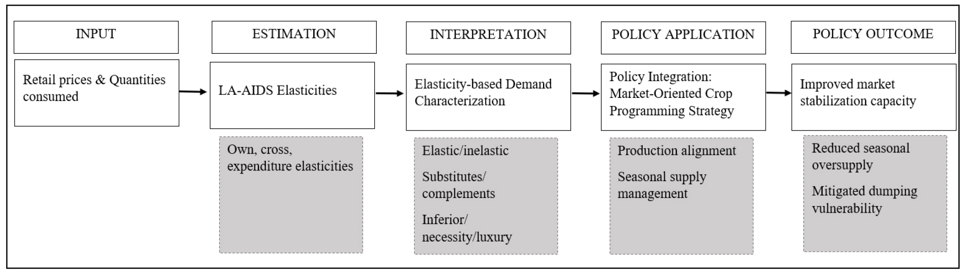
In the absence of systematic demand analysis, production decisions may contribute to synchronized planting and harvesting patterns that increase the risk of seasonal gluts. By aligning production decisions with anticipated market demand responsiveness, crop programming informed by elasticity estimates can enhance supply coordination, improve market stability capacity, and reduce vulnerability to dumping incidents. While demand elasticities alone cannot eliminate oversupply, they provide critical quantitative inputs for evidence-based agricultural planning.
Data and Methodology
Based on news media articles, the vegetables dominating dumping occurrences are cabbage, carrot, tomato, squash, and potato. The study uses the national quarterly consumption and national quarterly prices covering 60 observations from 2010 to 2024. Data on production, import, export, and prices are sourced from the OpenSTAT of the Philippine Statistics Authority (PSA). Data on post-harvest losses are sourced from different post-harvest articles and studies such as Key Player Perception on Postharvest Losses in the Highland Vegetable Value Chain (Launio et al., 2022) for cabbage, carrot and potato; and Analysis of Fruit and Vegetable Value Chain in the Philippines (Southeast Asian Regional Center for Graduate Study and Research in Agriculture, 2022) for tomato. There is no specific study or literature on postharvest losses for squash, other leafy vegetables, other legume vegetables, and other fruit vegetables, thus, this study utilizes the general average postharvest loss vegetables in the Philippines at 42% as cited by Mopera (2016).
National consumption of each vegetable under study (cabbage, potato, carrot, squash, tomato, other leafy vegetables, other legume vegetables, and other fruit vegetables) is computed as:
In specifying the demand system, the dependent variables are the budget shares allocated to vegetables. To ensure that the total vegetable expenditure is fully exhausted within the system, a residual category is incorporated to capture vegetables not explicitly modeled in the primary commodities. The classification of vegetable groups is guided by previously identified preferred or most-consumed vegetables in the literature, as well as by data availability.
To improve economic interpretability and reduce heterogeneity within groups, the residual category is organized into three economically meaningful subgroups: (i) other leafy vegetables, (ii) other legume vegetables, and (iii) other fruit vegetables. Based on consumption patterns reported in prior studies and the available dataset, there subgroups include: kangkong under other leafy vegetables; string beans (sitao) under other legume vegetables; and okra, eggplant, bitter gourd, and chayote under other fruit vegetables.
Although grouping commodities may introduce aggregation bias, where heterogenous price and substitution effects are averaged withing a composite category, this concern is moderated in the present context. Aggregation bias may attenuate cross-price relationships or smooth commodity-specific responses when individual items exhibit differing demand sensitivities. However, the vegetables included in these subgroups are not the primary focus commodities of the study but are incorporated to preserve the exhaustiveness of expenditure allocation and maintain theoretical consistency of the demand system. Accordingly, elasticity estimates for these aggregated subgroups should be interpreted with caution. This classification allows clearer identification of substitution and complementarity relationships across major vegetable categories while maintaining structural integrity of the LA-AIDS specification.
Empirical Model
The study employs the Linear Approximate Almost Ideal Demand System (LA-AIDS), originally developed by Deaton and Muellbauer (1980). The LA-AIDS simplifies the original nonlinear AIDS model by replacing the translog price index with a linear approximation, thereby facilitating estimation while preserving the theoretical properties of demand systems. The model provides a flexible framework for estimating price and expenditure elasticities while imposing adding-up, homogeneity, and symmetry restrictions.
The foundational demand system literature acknowledges the endogeneity challenges inherent in aggregate data (Deaton and Muellbauer, 1980), while temporal aggregation problem where high-frequency behavioral adjustments are observed only as period averages, has long been recognized in empirical demand analysis (Working, 1943). Moreover, as discussed by Griliches (1967), when behavioral adjustments occur at a higher frequency than the observation interval, data aggregation may obscure the underlying dynamic structure of economic relationships.
Consistent with this interpretation, lagged prices in this study should be understood as capturing short-run adjustment in aggregated demand data arising from contemporaneous endogeneity and temporal aggregation rather than demand inertia or state dependence. Incorporating lagged prices serves as a pragmatic reduced-form strategy to mitigate simultaneity and timing misalignment when valid external instruments are unavailable. The lagged-price LA-AIDS model expresses the budget share of a given good as a linear function of the logarithms of prices and real expenditure specified as:
The left side of Eq. (1) indicates the budget share of the ith commodity in period t defined as . The right hand of the equation includes the parameters αi, γij and βi, ρjt-1 as the price of commodity j in the previous quarter; X is the total expenditures on all vegetable commodities, and Pt is the price index.
While conventional LA-AIDS employs the Stone price index defined as:
this formulation uses contemporaneous budget shares as weights. Because the dependent variables enter directly into the construction of the price index, mechanical correlation between regressors and the disturbance term may arise. As noted by Moschini (1995), this feature may generate simultaneity bias and affect parameter consistency, particularly in small samples or when share volatility is substantial.
To mitigate this concern, the present study adopts a Laspeyres-type index with fixed base-period weights as the preferred specification. The index is defined as:
where represents the expenditure share of commodity i in a predetermined base period. Because these weights are fixed and predetermined, the Laspeyres index is not mechanically linked to contemporaneous demand shocks. This reduces simultaneity concerns while maintaining the linear approximation characteristic of the LA-AIDS framework.
For robustness, elasticity estimates are computed under alternative specifications: (i) contemporaneous prices, (ii) lagged prices with the Stone index, and (iii) lagged prices with the Laspeyres-type index. While most elasticities remain broadly stable across specification, the contemporaneous model yields a positive and statistically significant own-price responses for squash, whereas lagged specifications restore economically coherent own-price responses without attenuating price sensitivity for other commodities. We therefore associate the anomalous positive and significant own-price elasticity observed under the contemporaneous specification with contemporaneous endogeneity and timing misalignment in aggregated quarterly data, rather than with underlying consumer behavior. Furthermore, the Laspeyres-based specification exhibits slightly stronger theoretical regularity and more stable cross-price relationships.
Accordingly, the LA-AIDS model with lagged prices and the Laspeyres-type price index is adopted as the preferred specification, while the contemporaneous and Stone-based estimates are retained for robustness comparison. For transparency, the results of these alternative specifications are reported in the Appendix.
Restrictions implied by demand theory are imposed as follows:
Provided that these restrictions hold, the estimated demand functions add up to the total expenditure Eq. (2), are homogenous of degree zero in prices and income taken together Eq. (3), and satisfy Slutsky symmetry Eq. (4). (Hayes et al., 1990).
Because the vegetables’ expenditure shares () must sum to one, a demand system composed of the eight individual expenditure share equations would be singular. Therefore, one of the equations must be dropped to estimate the equations as a system. In this case, the ‘other fruit vegetable’ equation was chosen for deletion. However, the parameters for the omitted share equation can be calculated by using the adding-up restriction from Eq. (2).
In the AIDS model, each equation represents the demand for a specific good. However, the error terms in these equations can be related because the same factors may influence the demand for multiple goods at once. For example, an increase in a consumer’s income could affect how much they spend on both cabbage and carrot. To take these relationships into account, the Seemingly Unrelated Regression (SUR) method is used with homogeneity and symmetry restrictions imposed. This approach allows us to consider the correlations between equations, leading to more accurate and efficient estimates of the demand parameters.
The estimated parameters of LA-AIDS equation do not have straightforward economic interpretation but forms the basis of elasticity, which measures the percentage response of the budget share to a percent change in prices or total expenditure.
Elasticity Estimation
The estimated coefficients from SUR of the AIDS share equations are used to compute for the demand elasticities, which can quantify the price and expenditure responses of the consumers. The uncompensated (Marshallian) elasticities can be expressed as Eq. (5), (6), (7):
Where:
- expenditure coefficient from the AIDS estimation
- mean budget share for commodity i
- own-price coefficient
- cross-price coefficient
Summary Statistics and Parameter Estimation
Table 1 presents the descriptive statistics for the variables used in the study. Among the vegetables, the aggregated ‘other fruit vegetable’ has the highest consumer expenditure at 35%, while other legume vegetables have the lowest at 3%. For prices, squash has the lowest dispersion while potato exhibits the highest price variation. For budget share, the aggregated ‘other fruit vegetables’ has the highest mean budget share of 35%, while other leafy vegetable has the lowest at 8%.
Table 1
Descriptive statistics
The large standard deviations observed in the expenditure and price could be a reflection of seasonality and volatility of the vegetable market in the Philippines. Large variations in the commodity expenditures often corresponds to overproduction periods. Increased supply during certain months leads to price depression, which may contribute to dumping scenarios.
Table 2 summarizes the estimates coefficients for the budget share equation resulting from SUREG of AIDS to compute elasticities of the vegetables under study. The parameters include intercept (αi), expenditure parameter (βi), and price interaction parameter (γij) which forms the basis for deriving uncompensated elasticities to quantity consumer responsiveness to changes in price and income.
Table 2
Parameter estimates
| Parameter | Cabbage | Carrot | Tomato | Squash | Potato |
Other leafy vegetables |
Other legume vegetables | Other fruit vegetables |
|
-0.574 (0.388) |
-1.059** (0.499) |
-0.507 (0.794) |
0.309* (0.168) |
-0.547 (0.851) |
0.842*** (0.038) |
1.867*** (0.085) |
0.668 (0.952) | |
|
0.033* (0.020) |
0.057** (0.026) |
0.034 (0.041) |
-0.011 (0.009) |
0.032 (0.044) |
-0.041*** (0.002) |
-0.093*** (0.004) |
-0.012 (0.049) | |
|
-0.001 (0.018 |
0.017 (0.018) |
0.024 (0.024) |
-0.019* (0.010) |
0.018 (0.026) |
0.005** (0.002) |
-0.011* (0.006) |
-0.033 (0.032) | |
|
0.017 (0.018) |
0.035 (0.025) |
0.004 (0.030) |
0.020 (0.013) |
0.037 (0.034) |
-0.0003 (0.003) |
0.005 (0.007) |
-0.117*** (0.041) | |
|
0.024 (0.024) |
0.004 (0.030) |
0.023 (0.053) |
-0.019 (0.012) |
0.010 (0.050) |
-0.004 (0.003) |
-0.012* (0.006) |
-0.025 (0.054) | |
|
-0.019* (0.010) |
0.020 (0.013) |
-0.019 (0.012) |
0.049*** (0.017) |
-0.023* (0.014) |
-0.001 (0.003) |
-0.013** (0.007) |
0.006 (0.021) | |
|
0.018 (0.026) |
0.037 (0.034) |
0.010 (0.050) |
-0.023* (0.014) |
0.081 (0.058) |
-0.007** (0.003) |
-0.019*** (0.007) |
-0.097 (0.065) | |
|
0.005** (0.002) |
-0.0003 (0.003) |
-0.004 (0.003) |
-0.001 (0.003) |
-0.007** (0.003) |
0.008*** (0.002) |
0.0005 (0.001) |
0.0005 (0.004) | |
|
-0.011* (0.006) |
0.005 (0.007) |
-0.012* (0.006) |
-0.013** (0.007) |
-0.019*** (0.007) |
0.0005 (0.001) |
0.025*** (0.004) |
0.025*** (0.004) | |
|
-0.033 (0.032) |
-0.117*** (0.041) |
-0.025 (0.054) |
0.006 (0.021) |
-0.097 (0.065) |
-0.005*** (0.001) |
0.024*** (0.004) |
0.248*** (0.088) |
Results and Discussion
Before proceeding with the results and discussion, this study hypothesizes that price and expenditure elasticities provides a practical basis for crop programming; and that aligning production plans with market demand conditions may help mitigate supply glut and minimize risk of dumping. Specifically;
H1 (own-price elasticity):
H1a: Vegetables with inelastic demand are likely to be programmed for a stable production supply because price change does not have a major effect on demand.
H1b: On the other hand, vegetables having elastic demand should have a flexible planting production since demand reacts strongly to price change. In times of supply glut, elastic vegetables are prone to dumping.
H2 (cross-price elasticity):
H2a: Vegetables identified as substitute will compete for demand, therefore it needs stagger production. One substitute’s peak harvest should not also coincide with its substitute vegetable’s peak harvest.
H2b: In contrast, crops identified as complements may be programmed jointly to balance supply in the market.
H3 (Expenditure):
H3a: Vegetables which are considered as necessities will maintain a steady production across different income levels.
H3b: Inferior vegetables should avoid aggressive production expansion, maintaining only essential supply level since demand decreases as consumer income increases.
H3c: While for luxury vegetables, increase production only when market conditions are favorable.
Table 3 reports the estimated uncompensated (Marshallian) price elasticities and expenditure elasticities obtained from the Almost Ideal Demand System (AIDS) model. The own-price elasticities (diagonal elements in bold form) measure the responsiveness of demand to changes in each commodity’s own price, while the cross-price elasticities (off-diagonal) elements capture substitution and complementarity relationships among vegetables. The expenditure elasticities indicate how consumption patterns adjust as purchasing power changes, thereby identifying whether commodities behave as inferior, necessity, or luxury goods.
Table 3
Price and expenditure elasticities
| Price Elasticities |
Expenditure Elasticity | ||||||||
| Cabbage | Carrot | Tomato | Squash | Potato |
Others leafy veg |
Other legume veg |
Other fruit veg | ||
| Cabbage | -1.038*** (0.207) |
0.207 (0.214) |
0.289 (0.294) |
-0.232* (0.126) |
0.219 (0.316) |
0.056** (0.026) |
-0.130* (0.072) |
-0.403 (0.394) |
1.400*** (0.243) |
| Carrot |
0.240 (0.247) | -0.566 (0.350) |
0.053 (0.417) |
0.284 (0.177) |
0.527 (0.480) |
-0.004 (0.044) |
0.066 (0.101) |
-1.657*** (0.581) |
1.810*** (0.362) |
| Tomato |
0.136 (0.139) |
0.022 (0.170) | -0.903*** (0.323) |
-0.107 (0.068) |
0.058 (0.290) |
-0.023 (0.016) |
-0.071* (0.037) |
-0.146 (0.311) |
1.197*** (0.234) |
| Squash |
-0.257* (0.140) |
0.273 (0.170) |
-0.252 (0.161) | -0.323 (0.234) |
-0.312* (0.183) |
-0.020 (0.039) |
-0.180** (0.092) |
0.082 (0.280) |
0.854*** (0.118) |
| Potato |
0.118 (0.171) |
0.246 (0.224) |
0.067 (0.331) |
-0.152* (0.089) | -0.497 (0.376) |
-0.048** (0.019) |
-0.128*** (0.046) |
-0.638 (0.426) |
1.214*** (0.288) |
|
Others leafy veg |
0.158** (0.074) |
-0.011 (0.108) |
-0.136 (0.096) |
-0.050 (0.100) |
0.262*** (0.078) | -0.698*** (0.077) |
0.016 (0.047) |
-0.159*** (0.047) |
-0.415*** (0.067) |
|
Other legume veg |
-0.161* (0.090) |
0.070 (0.108) |
-0.186* (0.098) |
-0.201** (0.102) |
0.007 (0.020) |
0.382*** (0.055) | -0.525*** (0.055) |
0.359*** (0.060) |
-0.407*** (0.066) |
|
Other fruit veg |
-0.091 (0.091) |
-0.330*** (0.116) |
-0.066 (0.160) |
0.020 (0.060) |
-0.269 (0.181) |
0.002 (0.005) |
0.074*** (0.014) | -0.287 (0.255) |
0.966*** (0.139) |
These elasticity estimates provide critical evidence for market-oriented crop programming and agricultural policy design. These elasticities provide guidance on short-term market reactions to price movements, useful for quarterly crop programming and price policy simulation. In particular, understanding price responsiveness and substitution patterns allows policymakers to anticipate how consumers may adjust their consumption following price shocks, supply disruptions, or targeted interventions. Likewise, expenditure responsiveness offers insights into how rising incomes may shift demand toward specific vegetable groups, guiding production planning, resource allocation, and investment prioritization in the production side. Standard errors are reported in parentheses, and statistical significance is denoted at the 10%, 5%, and 1% levels.
The elasticity estimates are broadly consistent with economic demand theory, particularly with respect to the negative and statistically significant own-price elasticities observed for most commodities. The use of the Laspeyres price index and the incorporation of lagged prices appear to have contributed to obtaining theoretically plausible estimates by mitigating potential index number bias and short-run price endogeneity concerns. These specification choices strengthen confidence in robustness of the estimated demand responses and their suitability for policy simulation and crop programming applications.
Own-Price Elasticities (Short-Run)
The estimated own-price elasticities are all negative and the statistically significant coefficients are significant at 1% level, satisfying the theoretical requirement of downward-sloping demand. Interpreted as short-run adjustment elasticities due to the use of one-quarter lagged prices, the results indicate that vegetable consumption responds gradually to past price movements.
Cabbage exhibits an elastic short-run own-price elasticity of -1.038, implying that an increase in its price in the previous quarter reduces current demand by 1.038%. Tomato with a coefficient of -0.903, alongside other leafy vegetables (-0.698), and other legume vegetables (-0.525) also show relatively strong responsiveness. In contrast, although non-significant, squash (-0.323), potato (-0.497), and other fruit vegetables (-0.287) display more inelastic short-run responses, suggesting partial adjustment and greater consumption rigidity within a quarter. Overall, the magnitudes suggest that consumer responses to price changes are evident but not fully realized within a single quarter, which is consistent with the quarterly frequency of the data and the reduced-form dynamic adjustment embedded in the lagged-price specification.
Cross-Price Elasticities (Short-Run)
Table 3 further reports the statistically significant cross-price elasticities among vegetable commodities. Given the use of one-quarter lagged prices, these estimates should be interpreted as short-run adjustment effects, reflecting how current demand for one vegetable responds to price changes in another vegetable observed in the previous quarter. Positive cross-price elasticities indicate short-run substitutability, implying that an increase in the lagged prices of vegetable i leads to an increase in the current demand for vegetable j. Conversely, negative cross-price elasticities indicate short-run complementarity, suggesting that a rise in the lagged price of vegetable i reduces the current demand for vegetable j. At the 10% level of significance, the results identify squash-cabbage, other legume vegetables-cabbage, other legume vegetables-tomato, and squash-potato as complementary pairs. Stronger evidence of complementarity is observed for other fruit vegetables-carrot at the 1% level and other legume vegetables-squash at the 5% level of significance. Following the findings of Mutuc et al. (2007), the complementarity observed across broad vegetable categories may be due to the nature of how vegetables are cooked in the Philippines. That is, most of them are sauteed in oil or cooked together with some mixture of sauce, seasoning, or soup base. Many usual Filipino menus combine multiple vegetables, which may partly contribute to the complementarity.
Consistent still with the study of Mutuc et al. (2007), substitutability is primarily observed among vegetable commodities belonging to similar product groups. In the present study, at 5% level of significance, cabbage, a leafy vegetable, exhibits significant substitution effects with the residual variable ‘other leafy vegetables’, indicating competition within leafy vegetable consumption. Likewise, the aggregated categories ‘other legume vegetables’ and ‘other fruit vegetables’ demonstrate stronger substitutability at the 1% level of significance, further supporting the presence of within-group substitution patterns. However, due to the level of aggregation employed in constructing these residual categories, it is not possible to identify which specific vegetables within each subgroup drive the observed substitution effects. This aggregation may therefore mask commodity-specific demand relationships within the broader categories.
Expenditure Elasticity
The estimated expenditure elasticities indicate that most vegetables included in the analysis are classified as luxury goods (elasticity > 1), with coefficients statistically significant at the 1% level. By definition, a luxury good is one for which demand increases more than proportionally as total expenditure rises, implying that consumers allocate a larger share of their budget to these commodities as purchasing power expands. Consistent with the findings of Mutuc et al. (2007), cabbage is identified as a luxury good, both in earlier rural and urban estimates and in the present analysis. Conception (2009) likewise noted that higher-income households in Mindanao represent a potentially lucrative market for temperate vegetables such as cabbage, carrot, and potato. Note that these commodities are predominantly cultivated in high-altitude areas characterized by relatively cool year-round temperatures, with the Cordillera Administrative Region functioning as the country’s principal production hub and accounting for the bulk of national supply. The geographic concentration of production and the specific agro-climatic requirements of these temperate vegetables may contribute to limited supply responsiveness, thereby reinforcing their characterization as luxury goods in the consumption structure. Tomato, which Mutuc et al. (2007) previously classified as a necessity, now appears as a luxury good in the current estimates. This shift may reflect evolving consumption patterns over time, particularly given the nearly two-decade interval between the two studies. In contrast, squash and the aggregated category ‘other fruit vegetables’ are classified as necessities (0 < elasticity < 1), indicating that demand increases less than proportionally with rising expenditure. Meanwhile, ‘other leafy vegetables’ and ‘other legume vegetables’ exhibit negative expenditure elasticities and are therefore considered inferior goods. An inferior good is one for which demand declines as total expenditure or income increases, suggesting that consumers substitute away from these items toward relatively higher-valued alternatives as their purchasing power improves.
Application of Results to Crop Programming
The above elasticity results provide insights for crop programming by highlighting differences on how consumers respond to price and income changes, thus not all vegetable should be treated the same in terms of crop programming. However, demand elasticity estimates should be considered alongside production requirements. The estimated elasticities offer a conceptual basis for designing a demand-driven crop programming.
Supporting the initial hypothesis, vegetables with inelastic demand (other leafy vegetables, other legume vegetables, carrot, squash, potato, and other fruit vegetables) may benefit from established production quota to help maintain supply output to remain within the target range. Cabbage having an elastic own-price elasticity has a strong reaction to price change and is easily substituted when price increased. Overproduction of cabbage can increase the likelihood of unsold produce or dumping. Since demand increased more proportionally when price decreases, it may be advisable to expand production area during favorable production conditions. However, production expansion should be carefully planned based on market information to avoid glut.
Vegetables identified as complements (carrot-other fruit vegetables; other legume vegetables-squash; squash-cabbage; other legume vegetables-cabbage; other legume vegetables-tomato; squash-potato) may benefit from coordinate planting to jointly balance supply. Synchronized planting and harvesting can bring supply balance in the market since their demand tend to move together. A shortage of one crop (e.g., squash) may affect demand for its complement (e.g., cabbage), even when supply and price of the latter are stable. In this manner, the risk of having a supply glut of one vegetable while its complement faces shortage that may distort and weakens market demand for complement vegetables, will be reduced. For vegetable pairs exhibiting substitutability (cabbage-other leafy vegetables and other legume vegetables-other fruit vegetables), production planning may need to account for their competitive demand relationship. Because these commodities serve as substitutes, simultaneous market supply could intensify price competition, prompting consumers to shift toward the relatively cheaper option and increasing the risk of excess supply or price depression for the higher-priced commodities. Staggered production scheduling may therefore help mitigate direct competition within the same market window, reduce the likelihood of market gluts.
Vegetables classified as necessity, squash and other fruit vegetables, should maintain steady year-round production, as their demand do not drastically change with income changes, consumers purchase them regularly regardless of income level. The stable consumption means that a sudden expansion or contraction of production area can trigger market distortion. While vegetables classified as luxury (cabbage, carrot, tomato and potato), whose consumption rise more proportionally as income increases, may have a coincide harvest on high demand months or higher purchasing power. In the Philippines, high demand months includes December, when Christmas holiday spending, bonuses and other benefits are given, which may partly contribute to the increased food consumption. Other high-demand months include graduation month and regional festivals, in which demand typically spikes. Given that other leafy vegetables and other legume vegetables are classified as inferior goods, production expansion for these vegetables may be better targeted toward lower-income market segments or periods of constrained purchasing power, while cautious area allocation is advisable in anticipation of rising incomes, where demand may gradually shift toward higher-valued vegetables.
Overall, classifying vegetables according to their expenditure responsiveness (necessities vs. luxuries), price sensitivity (elastic vs. inelastic), and demand relationships (substitutes vs. complements) provide important demand-side insights for market-oriented crop programming. While elasticities alone cannot resolve structural supply imbalances, integrating these demand estimates with production planning can improve alignment between supply volumes and consumers’ willingness and ability to pay. Such coordination may contribute to reducing the risk of seasonal oversupply and price depressions that are often associated with vegetable dumping in the country.
Conclusion and Policy Recommendations
The study aims to determine demand elasticities of commonly dumped vegetables in the Philippines using the lagged-price LA-AIDS quantifying the consumer responsiveness to price and income changes. The findings of the study revealed that most vegetables have inelastic demand with cabbage as elastic and tomato as almost unitary elastic, mostly significant at 1% level. Vegetables show complementary relationship which may be due to nature of usual Filipino dishes while substitution relationship is observed between vegetables belonging to the same category like leafy vegetables. Most vegetables are classified as luxury significant at 1% in line with the findings of the previous study specifically for cabbage.
The estimated demand elasticities provide quantitative demand-side parameters that can be incorporated into the development of a market-responsive crop programming framework. By distinguishing vegetables according to their price sensitivity, income responsiveness, and inter-commodity relationships, planners can move beyond uniform production targets and adopt differentiated strategies that reflect actual market behavior. Elastic commodities require closer monitoring of production expansion to prevent price volatility, while inelastic commodities may allow relatively more stable output planning. Likewise, recognizing complementary and substitute relationships can guide coordinated or staggered planting decisions to reduce direct market competition and demand displacement.
The development of a more systematic, market-oriented crop programming framework has the potential to enhance welfare by helping reduce the frequency and severity of dumping episodes that contribute to price distortions and allocative inefficiencies during periods of oversupply. While elasticity estimates alone cannot prevent extreme supply gluts, integrating demand-side information into a coordinated market outlook system may support more informed planting and crop programming decisions at the beginning of the production cycle, rather than relying solely on past price signals or anecdotal expectations. Importantly, these elasticity estimates should be considered alongside supply-side factors such as production cycles, agro-climatic suitability, cost structures, and logistics capacity. Demand parameters alone cannot eliminate the structural causes of oversupply; however, their systematic incorporation into crop programming models may improve the alignment between production decisions and prevailing market conditions. In doing so, policymakers and planners may strengthen ongoing efforts to reduce recurrent seasonal gluts and enhance income stability among vegetable producers.
Future studies may expand this analysis into a fully integrated supply-demand framework of crop programming. While this paper provides the demand-side information on elasticity that quantifies consumer reaction in the market, a comprehensive conceptual model that combines these elasticities with actual production volumes can help support the crafting of a more market-aligned crop programming system of vegetables in the Philippines.
In addition, when data on actual volume of dumping is available, future studies may examine how dumping incidents affects consumption, demand elasticities, and the perceived prices of specific vegetables. Having an understanding whether dumping incidents depress demand or whether consumer respond opportunistically to low prices would add an important behavioral dimension to market analysis.
Lastly, regional demand analysis is recommended, recognizing the diverse vegetable preferences across different regions of the country due to differing food culture and local cuisines. Regional elasticities could help identify which areas can absorb specific vegetables in times of supply glut, enabling more targeted distribution strategies.
Appendix
Appendix Table 1
Price and expenditure elasticities using contemporaneous prices
| Price Elasticities |
Expenditure Elasticity | ||||||||
| Cabbage | Carrot | Tomato | Squash | Potato |
Others leafy veg |
Other legume veg |
Other fruit veg | ||
| Cabbage | -0.027 (0.178) |
0.050 (0.0203) |
-0.135 (0.255) |
-0.211** (0.090) |
0.350 (0.289) |
-0.042* (0.023) |
–0.219*** (0.054) |
-0.787** (0.391) |
1.260*** (0.258) |
| Carrot |
0.058 (0.235) | 0.106 (0.353) |
-0.253 (0.399) |
0.103 (0.134) |
0.162 (0.475) |
-0.086** (0.040) |
-0.280*** (0.085) |
-0.831 (0.600) |
1.289*** (0.413) |
| Tomato |
-0.064 (0.121) |
-0.103 (0.163) | -0.416 (0.268) |
-0.169*** (0.047) |
-0.220 (0.264) |
-0.022* (0.012) |
-0.065** (0.033) |
-0.110 (0.301) |
1.970*** (0.236) |
| Squash |
-0.234** (0.100) |
0.099 (0.129) |
-0.396*** (0.110) | 0.293** (0.148) |
-0.136 (0.113) |
0.028 (0.033) |
-0.155** (0.066) |
-0.484** (0.211) |
0.803*** (0.095) |
| Potato |
0.189 (0.156) |
0.075 (0.222) |
-0.252 (0.302) |
-0.066 (0.065) | -0.217 (0.368) |
-0.053*** (0.017) |
-0.140*** (0.044) |
-0.477 (0.414) |
0.609* (0.313) |
|
Others leafy veg |
-0.118* (0.064) |
-0.209** (0.099) |
-0.134* (0.072) |
0.072 (0.085) |
0.602*** (0.065) | -0.350*** (0.065) |
0.032 (0.043) |
-0.176*** (0.043) |
-0.649*** (0.060) |
|
Other legume veg |
-0.272*** (0.067) |
-0.301*** (0.091) |
-0.170** (0.087) |
-0.173** (0.073) |
0.014 (0.019) |
0.612 (0.047) | -0.274*** (0.048) |
0.438*** (0.048) |
-0.731*** (0.074) |
|
Other fruit veg |
-0.189** (0.089) |
-0.172 (0.119) |
-0.067 (0.149) |
-0.107** (0.045) |
-0.216 (0.176) |
0.0005 (0.006) |
0.110** (0.014) | -0.383 (0.298) |
1.073*** (0.161) |
Appendix Table 2
Price and expenditure elasticities using lagged prices with Stone’s price index
| Price Elasticities |
Expenditure Elasticity | ||||||||
| Cabbage | Carrot | Tomato | Squash | Potato |
Others leafy veg |
Other legume veg |
Other fruit veg | ||
| Cabbage | -0.977*** (0.206) |
0.233 (0.212) |
0.321 (0.283) |
-0.205 (0.126) |
0.252 (0.302) |
0.038 (0.029) |
-0.159** (0.076) |
-0.493 (0.371) |
0.875*** (0.255) |
| Carrot |
0.269 (0.246) | -0.414 (0.351) |
0.116 (0.406) |
0.278 (0.179) |
0.637 (0.467) |
-0.046 (0.049) |
-0.013 (0.111) |
-1.825*** (0.538) |
0.951** (0.388) |
| Tomato |
0.152 (0.134) |
0.047 (0.166) | -1.059*** (0.295) |
-0.120* (0.067) |
0.111 (0.267) |
-0.024 (0.017) |
-0.078* (0.044) |
-0.147 (0.279) |
1.682*** (0.225) |
| Squash |
-0.227 (0.141) |
0.267 (0.172) |
-0.281* (0.157) | -0.283 (0.236) |
-0.331* (0.185) |
0.024 (0.042) |
-0.098 (0.096) |
-0.075 (0.275) |
1.064*** (0.121) |
| Potato |
0.136 (0.163) |
0.297 (0.218) |
0.127 (0.306) |
-0.161* (0.090) | -0.356 (0.354) |
-0.076*** (0.022) |
-0.164*** (0.055) |
-0.730* (0.376) |
0.515* (0.290) |
|
Others leafy veg |
0.108 (0.081) |
-0.112 (0.121) |
-0.144 (0.101) |
0.062 (0.108) |
0.378*** (0.085) | -0.582*** (0.085) |
0.052 (0.055) |
-0.132** (0.056) |
-0.397*** (0.085) |
|
Other legume veg |
-0.197** (0.095) |
-0.014 (0.118) |
-0.205* (0.114) |
-0.110 (0.107) |
0.023 (0.024) |
0.440*** (0.063) | -0.470*** (0.063) |
0.378*** (0.067) |
-0.365*** (0.091) |
|
Other fruit veg |
-0.137 (0.085) |
-0.385*** (0.107) |
-0.119 (0.144) |
-0.036 (0.059) |
-0.355** (0.160) |
-0.003
(0.006) |
0.065*** (0.015) | -0.272 (0.238) |
1.269*** (0.139) |