Introduction

Salt removal from drainage water is becoming increasingly important for sustainable irrigated arid land agriculture where inadequate drainage infrastructure exists. Solar evaporation and concentration systems are currently in development in California for this purpose (Kim et al., 2007b). One technique under evaluation is an agricultural drainage water reduction system using a solar collector and a fire-tube boiler. This system can reduce a considerable amount of drainage water and leave residual salts at the bottom of the system. The remaining salts can be separated and recovered by pure salt products, such as NaCl, Na₂SO₄. Fundamentally, salt quality, production cost, and facility cost will be main issues for developing purified agricultural salt products. The recovery and separation of the salts should be investigated further.

A parabolic trough solar collector (PTC) is frequently employed for solar steam production (Kalogirou et al., 1997; Tuma et al., 1999; Fiedler et al., 2006), for power generation (Bakos et al., 2001; You and Hu, 2002), or for desalination (Kalogirou, 1998; Garcia-Rodriguez and Gomez-Camacho, 1999; Garcia-Rodriguez et al., 1999) because water temperatures of 300°C can be easily obtained without any decrease in the collector efficiency. Mathematical analysis of the PTC was performed (Edenburn, 1976; Kalogirou et al., 1994; Eskin, 1999) and efficiency evaluation was conducted (Tuma et al., 1999; Bakos et al., 2001; You and Hu, 2002; Pronobis, 2005). The analysis of the heat transfer in the boiler was performed as well (Godridge and Read, 1976; Heppenstall, 1993; Neshumayev et al., 2004).

In this study, simulation of the PTC and the boiler, prediction of the amount of water evaporated, and the calculation of the system efficiency will be performed separately. A comparison of the predicted results against experimental data will be presented. The economic analysis of the system will be conducted to help to determine the feasibility of utilizing this system as a farm scale plant.

The objectives of this task order are the performing technical modeling process for the boiler and the parabolic solar collector by creating computer simulation to predict technical performance. Furthermore the investigating the efficiency of the two systems and the preparing preliminary economic feasibility analysis for the boiler in terms of cost per dry salts produced.

Model development

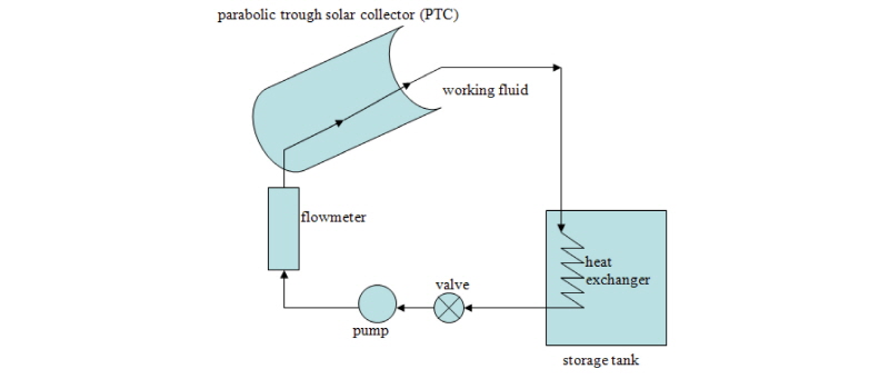
The system boundary of the PTC is the absorber pipe, the working fluid, and the heat exchanger which are coupled through heat exchange among them. The PTC and the boiler will be analyzed separately.

PTC

The collector consists of the cylindrical parabolic reflector and the absorber pipe. The absorber pipe is centered along the reflector’s focal line (Fig. 1). The temperatures of the absorber pipe are assumed to be uniform. The temperature gradients through the thickness of the walls of the absorber are assumed to be negligible. The working fluid is assumed to be completely in the liquid phase. The mass flow rate of the working fluid is considered to be constant and the heat transfer from the absorber pipe to the working fluid is convection only. Under the assumptions stated above and with the differential control volumes around the absorber pipe, the energy balances for the absorber pipe and the working fluid can be written as follows (Euh and Kim, 2013):

Fig. 1.

Systematic of parabolic solar collector (Euh and Kim, 2013).

Absorber pipe

       (1)

where,

A_a = absorber pipe area (m²)

k_a = thermal conductivity of the absorber pipe (W/m·°C)

T_a, T_w, and T_o = absorber, working fluid, and air temperature (°C)

τα = absorptance-transmittance product which varies with solar incident angle shown in Duffie and Beckman (1991)

γ_r = radiative reflection factor

I = solar intensity (W/m²)

w = reflector aperture (m)

d_ao and d_ai = outside and inside diameter of the absorber pipe (m)

h_w = convective heat transfer coefficient between the absorber pipe and the air= (W/m²·°C)

V = wind speed (m/s)

h_{r, sky} = radiative coefficient between the absorber pipe and the surroundings= (W/m²·°C)

ε_a = emissivity of the absorber pipe

σ = Stefan-Boltzman constant (5.6697×10^-8, W/m²·°C⁴)

T_sky = effective sky (lower atmosphere) temperature (°C) (Sartori, 1996)=

T_d = dew point temperature (°C)

ρ_a = density of the absorber pipe (kg/m³)

c_a = specific heat of the absorber pipe (J/kg·°C)

h_i = convective heat transfer coefficient between the working fluid and the absorber pipe (W/m²·°C)

                                                                             (2)

Nusselt number can be expressed with Reynolds number (Re) and Prantl number (Pr) (3).

                                                                    (3)

where,

L = length of the absorber pipe (m)

                                                                            (4)

where,

 = flow rate of the working fluid (kg/s)

μ_w = viscosity of the working fluid (kg/m·s)

Working fluid

                                                 (5)

where,

ρ_w, c_w, A_w = density, specific heat, and area of the working fluid (kg/m³, J/kg·°C, m²)

Heat exchanger

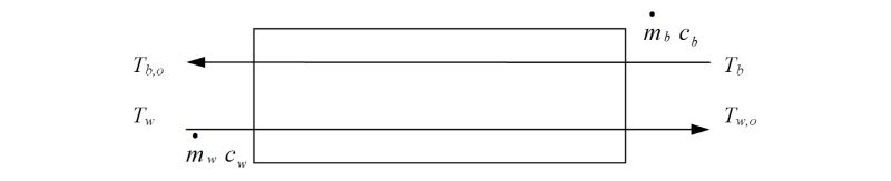
The rate of heat transfer between the two fluids in the heat exchanger is with appropriate temperatures and flows substituted in Fig. 2. The heat flow of the brine () can be expressed by (6, 7).

Fig. 2.

Heat exchanger.

                                                    (6)

Or,

 (Duffie and Beckman, 1991)                                           (7)

where,

T_w,o = Temperature of the working fluid out of the heat exchanger (°C)

T_b = Temperature of the brine into the heat exchanger (°C)

T_b,o = Temperature of the brine out of the heat exchanger (°C)

c_b = specific heat of the brine (J/kg·°C)

 = flow rate of the brine into the heat exchanger (kg/s)

 =

The heat exchanger effectiveness, ε, can be obtained from the various exchanger shapes (Kreith and Kreider, 1978). For the counter flow heat exchanger (Fig. 2):

                                                   (8)

                                                                   (9)

where,

                                                                           (10)

NTU = number of transfer units =                                                    (11)

where,

A = outside surface area of the heat exchanger (m²)

U_h = heat exchanger’s overall heat transfer coefficient (W/m²·°C)

 =

Boiler

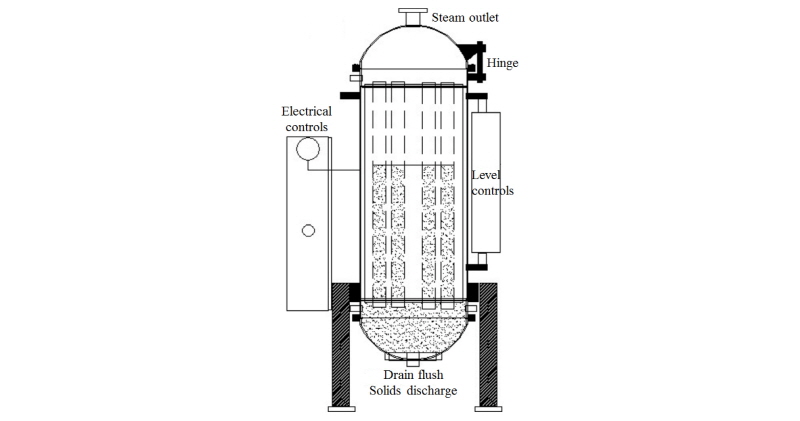
The boiler used in this study is a fire-tube boiler (Fig. 3). The flame for this type of boiler is short and enclosed in a small refractory chamber below a boiler shell containing water. The hot gas rises through vertical fire tubes passing through the shell. The thermal efficiency of these boilers is relatively low (50-65%).

Fig. 3.

Schematic of the boiler.

Flame temperature

The adiabatic flame temperature is a theoretical value depending on the excess air and the air preheat temperature. It can also be approximated based on a empirical relation (Basu et al., 2000):

                                                           (12)

where,

T_fl = theoretical adiabatic flame temperature (°C)

α_x = excess air coefficient (obtained from Basu et al. (2000), p. 36)

T_pre = preheat temperature of the combustion air (°C)

Heat transfer in a boiler

For radiative heat transfer between the flame and the fire tube is written as:

                                                                   (13)

where,

a_s = emissivity of the furnace wall-flame parallel planes system=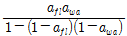

where,

a_wa = wall emissivity (1.0 (theoretically perfect black body, Kreith and Kreider, 1978))

a_fl = flame emissivity (0.9-0.95 (Basu et al., 1999))

F = fire-tube surface area (m²)

T_wa = furnace wall temperature (K)

To express the emitted radiation flux, J, of the flame, we use an overall furnace emissivity, a_fu, as follows:

                                                                            (14)

where,

J = radiation flux (W/m²)

a_fu = overall furnace emissivity =

ψ = thermal efficiency coefficient =

where,

x = angular coefficient (1.0 for boiler tube bundles (Basu et al., 1999))

ξ = fouling factor (0.65 for gas fuel (Basu et al., 1999))

The heat absorbed by the brine is only a part of the incident heat from the flame. The thermal efficiency coefficient is used to define the fraction of the outgoing radiation of the flame absorbed by the heating surfaces of the brine. The heat absorbed is written as:

                                                                  (15)

With equations (13) and (15), T_wa can be obtained:

                                                             (16)

where a_s is equal to a_fl when a_wa = 1. The heat absorbed by the brine from the furnace wall is by radiation and convection.

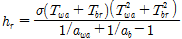
U = combination of radiative and convective heat transfer coefficients which is U = h_r + h_c.

                                                            (17)

where,

T_br = brine temperature inside boiler (°C)

a_b = brine emissivity (0.95 (Kreith and Kreider, 1978))

And,

                                                                            (18)

                                                 (19)

                                                                        (20)

where, 

k_b = thermal conductivity of the brine (W/m·°C)

L_t = tube length (m)

g = gravitational acceleration, 9.807 (m/s²)

β` = volumetric coefficient of expansion

ΔT = temperature difference between the furnce wall and the brine (°C)

ν_b = kinematic viscosity of the brine (m²/s)

α_b = thermal diffusivity of the brine (m²/s)

Total heat absorbed by the brine is:

                                                                  (21)

Under steady-state conditions, water evaporation rate is:

                                                                             (22)

where,

 = evaporation rate (kg/s)

h_fg = heat of vaporization (J/kg)

Solution procedure and model assumptions

Matlab v.6.5.0. (Mathworks, Inc, 2002) was used to solve the model equations. The specific heat of sea water was used for the brine specific heat. The temperature of feeding solution is assumed to be equal to the ambient air temperature when the parabolic trough solar collector is not operated due to the rain.

Results and Discussions

PTC

Prediction of absorber and fluid temperature

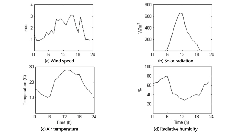
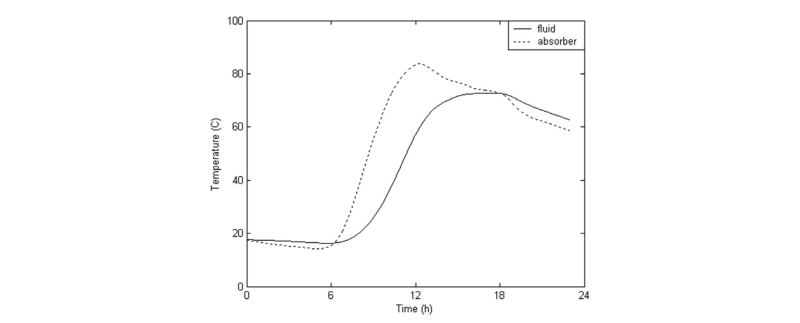
The system boundary of the parabolic solar collector was the absorber pipe, the working fluid, and the heat exchanger. The fire-tube type of boiler was used for this experiment. The energy and mass balance processes with finite differential approximation method was used to obtain fluid and absorber pipe temperatures of the solar collector and evaporation rates of the boiler. The simulation was performed using hourly CIMIS data (California Irrigation Management Information System, Department of Water Resources, http://wwwcimis.water.ca.gov/cimis) on May 3, 2006, at Five Points, California (Fig. 4). The calculated absorber pipe temperature went up to 85°C at noon due to the peak of the solar radiation. The fluid temperature was higher than the absorber temperature after 6PM. The fluid temperature differed from the absorber pipe temperature by as much as 15°C in the vicinity of maximum temperature (Fig. 5).

Fig. 4.

Ambient meteorological data. (a) wind speed, (b) horizontal solar radiation, (c) air temperature and (d) relative humidity.

Fig. 5.

Predicted fluid and absorbed temperatures of the parabolic solar collector.

Comparison experimental results with model predictions

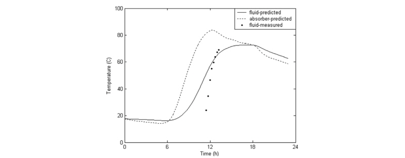
Experimental results were compared with predicted values under the same meteorological conditions. Fluid temperature was measured for 3 hours during daytime; it may not enough to compare measured and predicted results. However, the comparison of the peak fluid temperature and temperature variation can be performed and investigated. Predicted fluid temperatures followed the experimental results but deviated by more than 20°C when the experiment started. The reason for this deviation is due to the difference of the initial fluid temperature. The peak measured fluid temperature was 72°C which was close to the predicted results (Fig. 6).

Fig. 6.

Comparison of the measured and predicted fluid temperatures.

Boiler

The predicted wall temperature and the evaporation rate were compared with the measured results (Table 1). The measured wall temperature ranged from 218 to 288°C (425 to 550°F) and 76.0 kg of water per hour was measured to be evaporated which were in good agreement with model predictions (Table 1).

Table 1. Comparison of measured and predicted results for the boiler

Efficiency

PTC efficiency

A parabolic solar collector is inherently more efficient at a given temperature than a flat plate collector since the area from which heat is lost is smaller than the aperture area.

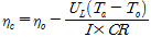                                                                   (23)

where,

η_c = thermal efficiency of the parabolic solar collector

η_o = optical efficiency (0.47-0.57 (Kalogirou et al., 1994))

U_L = heat loss coefficient (W/m²·°C)

I = solar beam radiation (W/m²)

CR = concentration ratio = A_a/A_r

A_L = aperture area (m²)

A_r = receiver area (m²)

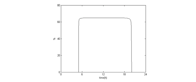
The calculated efficiency of the parabolic solar collector was approximately 64% during the daytime (Fig. 7).

Fig. 7.

Predicted efficiency of the parabolic solar collector.

Boiler efficiency

The efficiency of the boiler is defined as the ratio of the actual work to the negative of the enthalpy of combustion of the fuel. In this study, on the other hand, the efficiency of the boiler is defined by the relation such that:

                               (24)

where,

η_b = efficiency of the boiler

 = feeding brine flow rate (kg/h)

h_s = enthalpy of steam (kJ/kg)

h_b = enthalpy of feeding brine (kJ/kg)

 = fuel used rate (kg/h)

h_hv = higher heating value of fuel (kJ/kg)

The evaporation rate of the boiler was predicted to produce 82 kg/h and 70% of the boiler efficiency was calculated.

Economic analysis

Economic analysis for the boiler in terms of cost per dry salts produced was performed based on Present Worth Analysis and Equivalent Worth Analysis. In order to obtain cost per dry salts, two methods was used as follows:

(1) Find the Net Present Worth for the project and divide it by the total salts produced over the project’s life.

(2) Find the Annual Equivalent Worth for the project and divide it by the amount of salts produced per year.

Assumptions

Table 2. Boiler characteristics and costs

Boiler capacity was determined based on the prototype boiler tested in this study. Under the assumption of 1 m³ of natural gas used per month ($300 m^-3; http://www.eia.doe.gov/oil_gas/natural_gas/info_glance/natural_gas.html), the operation and maintenance cost for one prototype boiler is ($3,600 year^-1 gas) + ($5,000 year^-1 maintenance). The other boilers can produce 2, 5, and 10 times more salts than the prototype boiler, and the same as natural gas spent. The maintenance cost is fixed.

Net Present Worth analysis

Net present worth (NPW) can be calculated by computing the present worth of cost for the ten years:

Present Worth = (P/F,i,n) =                                                        (25)

where,

P = present sum

F = future sum

i = interest rate

n = project life (years)

NPW = $2,500 (boiler) + 8,600 (P/F, 8%, 1) + 8,600 (P/F, 8%, 2) + 8,600 (P/F, 8%, 3) + ··· + 8,600 (P/F, 8%, 10) = $60206.70.

Thus, the cost per dry salts for the prototype boiler is:

Cost per dry salts kg^-1 salt

where, Q = quantity of salts produced per year.

The costs per dry salts for the rest of boilers in terms of NPW were in the Table 3.

Table 3. Cash flows for this study (unit: $)

Equivalent Worth analysis

With the NPW known, the equivalent uniform annual cost (EUAC) can be computed using the capital recovery factor as follows:

EUAC = NPW (A/P, 8%, 10)                                                                (26)=

Cost per dry salts kg^-1 salt

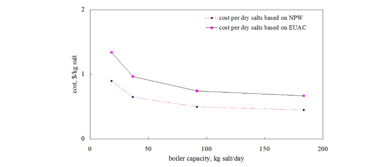
The variation of the costs per dry salts for all boilers in terms of boiler capacity is in the Fig. 8.

Fig. 8.

Cost per dry salts produced in terms of boiler capacity.

Conclusions

Salt management in irrigated agriculture is critical to the economies of the San Joaquin Valley of California and many other areas around the world. Purified salts can be recovered as marketable products through fractional crystallization following concentration of final stage drainage water from integrated on-farm drainage management systems (IFDM, Cervinka et al., 1999). To obtain recovered salt and use as a commercial product, new systems which can perform with higher efficiency and lower environmental impact than solar evaporation basins or solar ponds that have previously been used for the final stage are in need of development (Kim et al., 2007a). For this purpose, a boiler-assisted brine concentration system has been investigated including mathematical simulation along with an economic feasibility analysis. Model performance was conceptually evaluated and then experimentally verified.

A transient model was developed from energy and component mass balances and employed constitutive heat and mass transfer relationships from various other sources for simulating concentration of agricultural drainage water using the boiler and the parabolic solar collector separately.

The model of the parabolic solar collector yielded good predictions relative to experiments in terms of fluid temperature change and peak fluid temperature. The deviation between the calculated and measured fluid temperatures was more than 20°C at starting point due to the different initial fluid temperature. The peak temperature measured by 72°C was close to the calculated results. The evaporation rate of the boiler was 82 kg/h from the model prediction and 76 kg/h from the measurement. The predicted efficiencies of the parabolic solar collector and the boiler were approximately 64% during the daytime, and 70% respectively.

The cost per dry salts based on NPW for the prototype boiler was $0.90 kg^-1 salt and $1.34 kg^-1 salt based on EUAC respectively, and the costs were decreased as the boiler capacity was increased. However, there exist a couple of variables which can change the economic analysis results such as the operation and maintenance cost and the boiler life. Further economic investigation needs be performed.