

Introduction
Materials and Method
Materials
Pearson correlation coefficient
Model development and evaluation
Results and Discussion
Pearson correlation between variables
Calorific value prediction model development based on elemental analysis
Calorific value prediction model development based on proximate analysis
Calorific value prediction model development based on chemical composition analysis
Calorific value prediction model validation
Compared with previous models
Conclusions
Introduction
In recent years, one of the most pressing global concerns has been the energy crisis, which is primarily being driven by rapid climate change caused by fossil fuels (Gajdzik et al., 2024; Hussain et al., 2023). To address this issue, many countries have actively promoted for the use of alternative fuel sources, such as agricultural leftovers utilised as biomass fuel for heating and power generation (Bistline et al., 2023; Dinu, 2023; Ministry of Trade, Industry and Energy, 2023; Nam, 2020). The benefit of using such fuels for small-scale combustion or thermochemical conversion is clear, as the fuels are renewable resources that offer a cost-effective supplementary fuel source. Furthermore, this application provides an opportunity to solve the issue of waste disposal.
Previously, numerous studies have been conducted to develop models for predicting the calorific value of solid fuels using different analytical approaches. Using elemental analysis, models for forecasting calorific values were first based on coal rather than biomass. As a result, numerous models for forecasting calorific values using elemental analysis were developed, with coal serving as the reference material (Singh and Kakati, 1994). Dulong’s formula, a well-known equation calculated using elemental analysis, is routinely used to assess the calorific value of coal. When compared to data acquired using an oxygen-bomb calorimeter, it can provide reliable estimates of the calorific value for anthracitic, semi-anthracitic, and bituminous coals with an error margin of about 1.5% (Lowry, 1963). Several scholars then developed calorific value prediction models for coal (Mendeleev, 1897; Schuster, 1931; Steuer, 1926). For proximate analysis, de KOCK and Franzidis (1973) proposed a prediction model based on South African coal from a prior study. An equation using moisture content, volatile matter, fixed carbon, and ash was proposed, which included squares and cubes. Ebeling and Jenkins (1985) conducted a variety of analyses, including proximate analysis, elemental analysis, and caloric value. Various equations were proposed for different types of biomass (field crops, orchard pruning, vineyard pruning, energy crops, forest waste, etc.). ÖzyuǧUran and Yaman (2017) proposed calorific value prediction models based on proximal analysis. It stated that accurate forecasts can be produced when the biomass has a calorific value more than 20 MJ/kg. Also, a prediction model based on chemical composition analysis was developed. Howard (1973) researched the variance in calorific values across different portions of pinewood and discovered a link between extractives and calorific values. Tillman (1978) used a single variable in a model to calculate the higher calorific value (HHV) of wood, expressed in both dry weight and dry ash-free (DAF) terms. White (1987) presented four equations. One of these equations was created for wood having extractives, whereas the other three were meant for diverse types of wood that did not include extractives. Subsequently, several research were done and described in Table 1. The above previous studies have focused on general biomass, whereas research specifically addressing agricultural residues, particularly biomass subjected to torrefaction, remains limited.
Table 1.
Previous prediction model using elemental, proximate, chemical composition analysis
| Equation | Year | Fuel | Ref. |
| Elemental analysis | |||
| 1926 | Coal | (Steuer, 1926) | |
| 1994 | Coal | (Singh and Kakati, 1994) | |
| 2002 | Any fuel | (Channiwala and Parikh, 2002) | |
| 2005 | Biomass | (Friedl et al., 2005) | |
| 2005 | Biomass | (Sheng and Azevedo, 2005) | |
| 2020 | Biochar | (Qian et al., 2020) | |
| 2022 | Torrefied biomass | (Parnthong et al., 2022) | |
| Proximate analysis | |||
| 1985 | Field crop | (Ebeling and Jenkins, 1985) | |
| Vineyard pruning | |||
| Forest residues | |||
| Wood | |||
| Biomass | |||
| 1991 |
Lignocellulosic residue | (Jiménez and González, 1991) | |
| 1997 | Biomass | (Demirbaş, 1997) | |
| 2001 |
Raw and thermal treated lignocellulosic residue and | (Cordero et al., 2001) | |
| 2018 |
Lignocellulosic residue | (Krishnan et al., 2018) | |
| 2018 | Sugarcane residue | (Conag et al., 2019) | |
| 2020 | Biochar | (Qian et al., 2020) | |
| 2020 | Biomass | (Roy and Ray, 2020) | |
| Chemical composition analysis | |||
| 1973 | Pine | (Howard, 1973) | |
| 1978 | Extractive-free wood | (Tillman, 1978) | |
| 1984 |
Unextracted wood, Four softwoods and four hardwoods | (White, 1987) | |
| Extractive-free wood | |||
|
Extractive-free softwood | |||
|
Extractive-free hardwood | |||
| 2001 |
Extractive-free wood and non-wood | (Demirbas, 2001) | |
|
Extractive-free lignocellulosic materials | |||
|
Extractive-free non-wood | |||
| 2015 |
Agro-forestry wastes and industrial wastes | (Álvarez et al., 2015) | |
| 2019 |
Tree Species from Oaxaca, Mexico | (Ruiz-Aquino et al., 2019) | |
| 2020 |
Mixture of eight untreated and heat-treated woods | (Domingos et al., 2020) | |
Where, C, H, N, O, S, VM, FC, Ash, [C], [H], [L], [L*], [E] and [Ho] stand for carbon, hydrogen, nitrogen, oxygen, sulphur, volatile matter, fixed carbon, ash, cellulose, hemicellulose, lignin, extractive-free lignin, extract, and holocellulose, respectively. The superscript B indicates that the unit is British BTU.
This work concentrated on empirical correlations that used elemental, proximate, and chemical composition investigations of torrefied lignocellulosic biomass components to estimate HHV. The accuracy of these correlations was compared to current HHV correlations using biomass. These newly established correlations provide a simpler, more cost-effective, and faster way to forecast HHV of torrefied agricultural biomass. The models are especially useful for researchers who do not have access to expensive or sophisticated equipment for experimental HHV determination.
Materials and Method
Materials
Previous research findings were used to construct this model (Park et al., 2024). It was summarised in Table S1. Agricultural biomass including corn cobs, bean pods, pepper stems, grape pruning branches, wood pellets and bamboo were utilised. Soybean pods and corncobs were purchased from Hanjung SS Co., Ltd., Seoul, Korea. The biomass kinds were all represented as feed pellets. To produce woody agricultural biomass, pepper stems and grape pruning branches were collected from local farms in Gochang-gun, Chungcheongnam-do, and Paju-si, Gyeonggi-do, Korea. Wood pellets came from the Yeoju Forestry Association in Yeoju-si, Korea. Korea Bamboo Co., Ltd., situated in Hapcheo-gun, Gyeongsangnam-do, Korea, delivered at least three years of bamboo. The torrefaction process was done with 75 mm diameter and 55 mm high stainless steel cans and an electric furnace (N7/H/B410, Nabertherm GmbH, Germany). There was 100 ± 2 g of material in each of the stainless steel cans. Parts of 50 ± 2 g were used for BB, though, because of volume concerns. At 30 minute and hourly intervals, the process was done at temperatures between 230 and 310°C and 20°C. The samples were given names based on their processing time and temperature. For example, the CC23030 sample was heated to 230°C for 30 minutes.
The range of biomass resulting from elemental analysis is shown below: Carbon ranged from 38.63% to 69.87%; hydrogen from 4.01% to 6.25%; and oxygen from 24.68% to 53.71%. For proximate analysis, volatile matter (VM) ranged from 30.58% to 82.96%, while fixed carbon (FC) and ash content ranged from 16.42% to 63.51% and 0.13% to 16.30%, respectively. Chemical composition research revealed that cellulose content ranged from 1.09% to 47.91%, whereas hemicellulose content ranged from 0% to 43.10%. Lignin content had the greatest variation, ranging from 10.50% to 89.78%. The calorific value ranged from 17.44 to 28.03 MJ/kg. The total number of data points was 66. Linear regression analyses were carried out using IBM SPSS version 22.0, yielding correlation equations with variable goodness of fit values. In this study, data was analysed using the SPSS software’s “stepwise” and “enter” procedures. Although various recent studies have applied advanced techniques such as artificial intelligence (Mondal and Rafizul, 2025), linear regression offers the advantage of being simple and directly applicable. For this reason, the present study employed a linear regression model.
Pearson correlation coefficient
The correlation between calorific value results, proximity (VM and FC), composition (Cell, Hemi, and Lig), and a range of elements (C, H, N, O, and S) was investigated using the Pearson correlation coefficient (Eq. (1)). Two populations’ degree of association was ascertained using the Pearson correlation coefficient—defined in equation 1. It runs from -1 to 1; positive and negative values indicate a proportional and inverse connection, respectively. Values around -1 or 1 show a higher linear correlation; values near 0 show a lower correlation (Park et al., 2023). Linear and nonlinear regressions on the final analytic data using IBM SPSS version 22.0 produced correlation equations with varying goodness of fit scores.
Model development and evaluation
Four performance metrics were employed to assess the appropriateness of the models (Eq. (2),(3),(4),(5)). These metrics include the coefficient of determination (R2), root mean squared error (RMSE), average absolute error (AAE), and average bias error (ABE). The performance metrics equations were as follows:
Where, n and i defined as the number of samples and the initial sample number, respectively. Subscription P and M refers prediction and measure, respectively.
For selecting optimal model, validation was conducted using data from previous data (Chen et al., 2011a, 2011b; Li et al., 2015; Lyu et al., 2015; Ma et al., 2019; Meng et al., 2012; Peng et al., 2012; Rodriguez Alonso et al., 2016; Rousset et al., 2011; Wang et al., 2018, 2021; Yang et al., 2015). Validation data is summarized in Table S2. Also, the data for Table S2 was used for comparison with selected optimal model and previous study model.
Results and Discussion
Pearson correlation between variables
Fig. 1 exhibits the results of the Pearson correlation coefficient. In the correlation between elemental analysis (C, H, N, S, O) and calorific value, N and S had modest correlations of 0.07 and -0.27, respectively. In contrast, carbon, hydrogen, and oxygen were discovered to have strong positive or negative connections. A high positive association was found for carbon. This was because the calorific value rose with the carbon content during the torrefaction process. On the contrary, hydrogen and oxygen levels fell due to devolatilization throughout the torrefaction process, while calorific value increased, indicating a negative association. In the case of proximal analysis, the VM demonstrated a substantial negative correlation of -0.76. On the other hand, the FC had a substantial positive correlation of 0.89. The ash content indicated a weak negative correlation (-0.11). As the torrefaction process progressed, the calorific value and FC rose, resulting in a significant positive connection. Volatile matter showed a substantial negative correlation as it decreased. There was a significant difference in ash concentration depending on the sample (e.g., herbaceous biomass and woody biomass), however a slight negative connection was found because combustible matter rose as ash content decreased, resulting in a high calorific value. For chemical composition, cellulose and hemicellulose showed negative correlations of -0.87 and -0.64, respectively, while lignin showed a strong correlation of 0.94. As the torrefaction process progressed, cellulose and hemicellulose decomposed rapidly, but lignin decomposed at a relatively high temperature, resulting in a larger content than cellulose and hemicellulose. Based on this, it was determined that C, H, and O in elemental analysis, VM and FC in proximate analysis, and cellulose, hemicellulose, and lignin in chemical composition all had a substantial link with the calorific value.

Calorific value prediction model development based on elemental analysis
Table 2 summarises the models used to forecast calorific value based on elemental analysis data. Although E2, with the greatest R2P of 0.9652, had the most elements as input variables, there was no significant difference between it and E1, which had an R2P of 0.9632. The performance gap between E2 and E1 in R2 was marginal, suggesting that adding more input variables in E2 did not yield a substantial improvement over E1. This may be due to the relatively high intercorrelation among elemental parameters such as C, H, and O contents in the dataset, which can limit incremental gains from additional variables. In comparison, E3 showed a relatively high R2P of 0.9302 but was the lowest of the three predictive equations. The lower performance of E3 can be attributed to its reduced variable set, which likely omits key elemental predictors directly correlated with carbon content and energy density. Among the three equations, E2 had the lowest R2P, as well as the lowest RMSEP, AAEP, and ABEP, with values of 0.4544, 1.8333, and 0.0400.
Table 2.
Summary of proposed model using elemental analysis
| No. | Proposed models |
R2P (-) |
RMSEP (MJ/kg) |
AAEP (%) |
ABEP (%) |
| E1 | 0.9632 | 0.4677 | 1.8971 | 0.0974 | |
| E2 | 0.9652 | 0.4544 | 1.8333 | 0.0400 | |
| E3 | 0.9302 | 0.6437 | 2.5064 | 0.0690 |
Calorific value prediction model development based on proximate analysis
Table 3 highlights the models for projecting calorific values based on proximal analysis. These models had lower R2P values than those obtained from elemental analysis (E1–E3). It reflected the fact that proximate composition were indirect indicators of calorific value and less precise than elemental composition in representing calorific value. Out of these models, P2 with two input variables outperformed P1 on all four performance criteria (R2P, RMSEP, AAEP, ABEP).
Table 3.
Summary of proposed model using proximate analysis
| No. | Proposed models |
R2P (-) |
RMSEP (MJ/kg) |
AAEP (%) |
ABEP (%) |
| P1 | 0.7882 | 1.1218 | 4.5587 | 0.3446 | |
| P2 | 0.8858 | 0.8238 | 3.4100 | 0.1429 |
Calorific value prediction model development based on chemical composition analysis
The method for predicting heating value using chemical composition analysis is presented in Table 4. Both equations include lignin as a predictor variable because lignin has a high carbon content and tends to increase during high-temperature processing, which directly contributes to higher HHV. In the case of S1, the R2P (0.8892) was significantly lower than that of S2 (0.9082). This performance gap may be due to S2 incorporating an additional structural carbohydrate term, allowing it to capture more variance in the calorific value.
Table 4.
Summary of proposed model using chemical composition analysis
| No. | Proposed models |
R2P (-) |
RMSEP (MJ/kg) |
AAEP (%) |
ABEP (%) |
| S1 | 0.8892 | 0.8116 | 3.1450 | 0.0307 | |
| S2 | 0.9082 | 0.7386 | 2.8467 | 0.0179 |
Nevertheless, S1 achieved a higher R²P than the proximate analysis-based models (P1, P2), indicating that chemical composition parameters, particularly lignin, are more strongly correlated with HHV than proximate variables such as volatile matter and ash. For RMSEP, AAEP, and ABEP, S2 outperformed S1, suggesting that its expanded variable set improved calibration accuracy.
Both models had positive ABEP values, implying slight underestimation of HHV. This bias may be due to a high proportion of high-HHV samples in the dataset, which positioned the regression line slightly below the ideal 1:1 line—leading to conservative predictions. While this reduces overestimation risk, it can limit accuracy when predicting upper-bound HHV values.
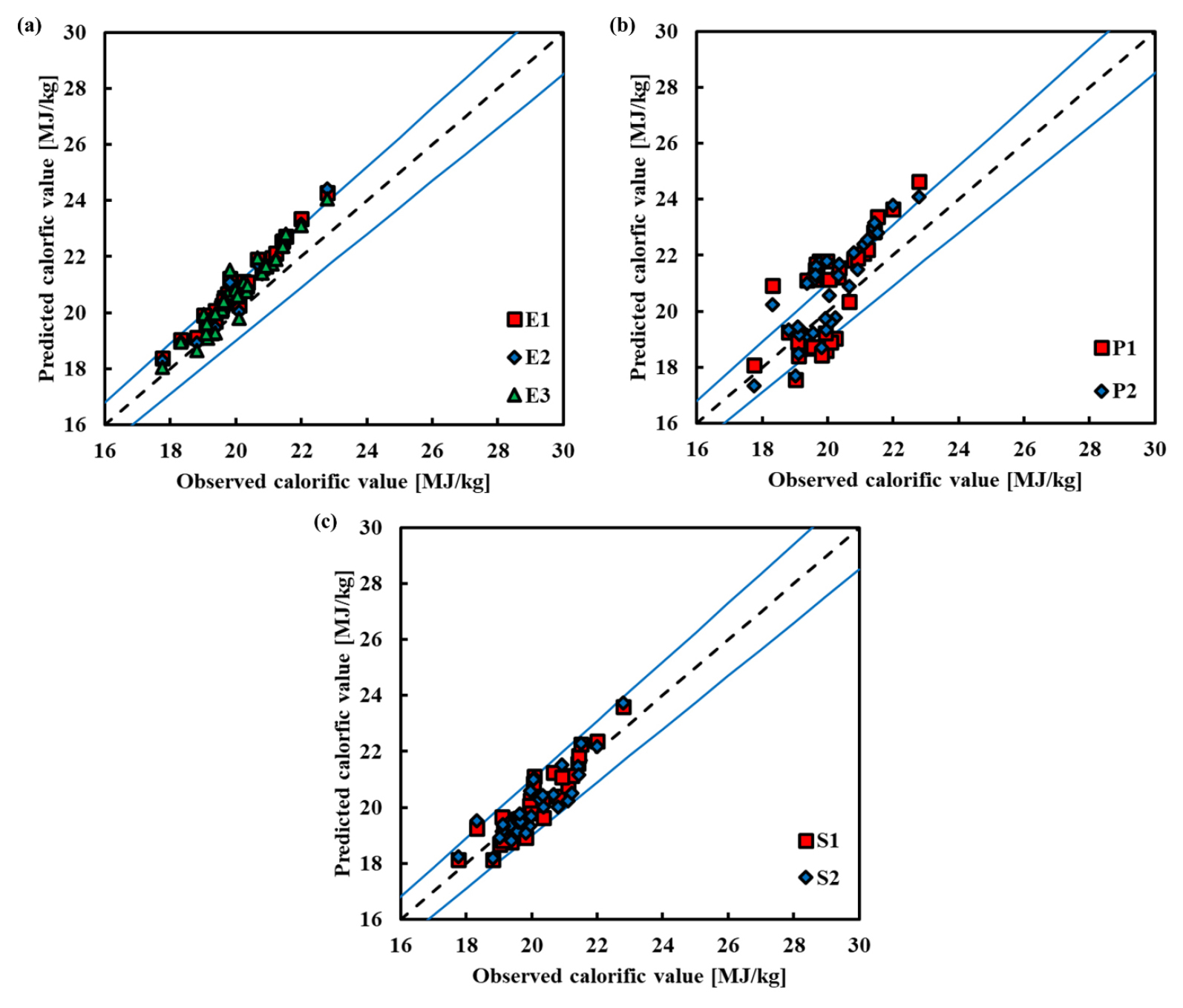
Calorific value prediction model validation
The data provided below was utilised to confirm the equations obtained from elemental analysis, proximate analysis, and chemical composition analysis (Table S1). All results are reported in Table 5.
Table 5.
Validation results of each model
For equations predicted by elemental analysis, E1 had the lowest RMSEV of 0.8416 and the greatest R2V of 0.9660. E3 and E2 exhibited RMSEV values of 0.7685 and 0.7134, respectively. However, despite E2 having a lower RMSEV than E1, its R2V was incorrectly reported as 0.578 in the original text and is actually much lower than expected when compared to E3 (0.9233). This discrepancy suggests possible inconsistencies in the validation data or calculation, which should be clarified. Fig. 2(a) shows that the prediction values from all prediction models were grouped closely together. E1 was determined to be the best fit because it achieved the most balanced trade-off between accuracy and generalisation, indicating that a simpler variable set can sometimes yield more robust predictions when predictor variables are highly correlated.
For equations predicted by proximate analysis, P1 had an RMSEV of 1.1035, but P2 had a lower RMSEV of 1.0243. Nevertheless, both models exhibited substantially lower R2V compared to those based on elemental or chemical composition analysis, which confirms that proximate variables are less directly correlated with HHV. In Fig. 2(b), P2 appeared closer to the 1:1 middle line than P1, indicating a slightly better alignment with actual values. However, the relatively high residual spread in both models suggests that proximate analysis alone may not capture sufficient variability in HHV, especially for heterogeneous biomass samples. Because of its higher overall performance metrics, P2 was chosen as the best model for forecasting calorific value using proximate analysis.
S1 and S2 had RMSEV values of 0.8549 and 0.7896, respectively. S2 had a greater ABEV than S1, although the AAEV was lower in S1. This pattern indicates that while S2 reduced average absolute error, it introduced a systematic positive bias—overestimating HHV more often—possibly due to overfitting during calibration. As illustrated in Fig. 2(c), predictions of S1 were more evenly distributed around the 1:1 line, resulting in lower bias and greater robustness across the validation set. Therefore, despite lower RMSEV of S2, S1 was considered the better model because it offered more balanced and generalisable performance.
Compared with previous models
In order to compare the model presented in this study with previous studies, predictions were made using validation data in Table S2. In the case of elemental analysis, equations were compared with previous models from Parnthong et al. (2022) and Qian et al. (2020). Two models were used for comparison because both were prediction equations based on heat-treated biomass. For predictions derived from proximate analysis, those suggested in this studies were compared with the equations proposed by Demirbas, and Sheng and Azevedo, which were generally used (Demirbaş, 1997; Sheng and Azevedo, 2005). As for predictions based on chemical composition analysis, there were many similar equations from previous research using similar samples, such as Álvarez et al. (2015) and Domingos et al. (2020). The compared data are based on the information in Table 6 and Fig. 3(a). When elemental analysis was used, E1 exhibited a higher R2 than the two equations from previous studies, although Qian et al. showed a slightly higher RMSE. R2 of Parnthong et al. showed the lowest performance, showing 0.6570. The graph indicates that the results from Parnthong et al. were scattered. E1 and Qian seemed to follow the reference line closely. When predictions were made based on proximate analysis (Fig. 3(b)), proposed equation in this study, P2, showed the lowest RMSE of 1.0243. The results from all the equations on the graph were generally scattered. Sheng and Azevedo’s results indicated a slight increase in trend as observed heat values increased. For predictions based on chemical composition analysis (Fig. 3(c)), all models exhibited an R2 of 0.8549. In the case of S1 and Domingos et al., it appeared close to the reference line, but in the case of Álvarez et al., it appeared linear at the bottom. Domingos et al. showed the lowest RMSE, 0.6144, but the RMSE of S1, the model presented in this study, was 0.6201, showing no significant difference.
Table 6.
Comparison results with previous prediction models
Conclusions
This work sought to construct appropriate equations for determining heating values depending on elemental composition, proximal analysis, and chemical properties of biomass produced by pyrolysis. Data obtained from the study of agricultural wastes, together with their elemental, proximal, and chemical composition characteristics, was used to build the prediction models.
The kind of analysis done affected the correctness of the heating value equations. Whereas those from proximal and chemical composition analyses showed R2P values between 0.7882 and 0.9882 and 0.892 to 0.9082, respectively, the coefficients of determination (R2P) for models based on elemental composition ranged from 0.9302 to 0.965. Among these, the least accurate prediction equations came from proximal analysis. Finding the most trustworthy models for any analytical method depended much on validation techniques. After validation, the suggested equations were validated by matching with earlier research. According to the results, for heating values the created models either perform as well as, or better than, past predictive models.
It is important to highlight that this study only examined agricultural biomass. Future studies should use elemental and proximal assessments to a wider spectrum of biomass forms, including coal and municipal solid waste (MSW). Furthermore, improving the general accuracy and applicability of these equations is including a more varied range of lignocellulosic biomasses into chemical composition-based prediction models. These equations can be used in many practical instances, such as choosing the best feedstock and process conditions for industrial bioenergy production, making better use of resources in agricultural waste management, and giving trustworthy information to help policymakers make decisions about deploying renewable energy.
