Evaluating Technological Progress and Energy Consumption in Korean Agricultural Sectors: An Application of the Autoregressive Distributed Lag Model Approach

Hoyeon Jeong

doi:10.22698/jales.20240034

Preview

Research Article

Journal of Agricultural, Life and Environmental Sciences. 31 December 2024. 446-458
https://doi.org/10.22698/jales.20240034

Evaluating Technological Progress and Energy Consumption in Korean Agricultural Sectors: An Application of the Autoregressive Distributed Lag Model Approach

Hoyeon Jeong¹^*

¹Postdoctoral Scholar, Department of Agricultural Economics, University of Kentucky, Lexington, Kentucky, 40546, United States

^{*Corresponding Author}

License (open-access, https://creativecommons.org/licenses/by-nc/4.0/):

This is an Open-Access article distributed under the terms of the Creative Commons Attribution Non-Commercial License (https://creativecommons.org/licenses/by-nc/4.0) which permits unrestricted non-commercial use, distribution, and reproduction in any medium, provided the original work is properly cited.

ABSTRACT

This study investigates the relationship between energy consumption, technological progress, value-added agriculture, and arable land in the Korean agricultural sector. We introduce an Autoregressive Distributed Lag (ARDL) model to examine the short- and long-run relationships among variables using a bounds test. We found that an increase in agricultural Total Factor Productivity (TFP) is associated with a 0.021% decrease in energy consumption in the agricultural sector in the long run. Moreover, we confirm the Kuznets curve hypothesis, in which the relationship between energy consumption and economic growth in the agricultural sector shows an inverted U-shape. This means that energy consumption increases at the initial stage of economic development in the agricultural sector but eventually decreases at a later stage. Finally, we confirmed that the expansion of arable land leads to an increase in energy consumption in the short run, whereas the relationship is reversed in the long run. This may have resulted from a decreasing trend in the arable land size used for Korean agricultural production. Our findings will help policymakers develop educational programs for farmers to enhance their productivity and use energy sources efficiently.

Keywords

Agricultural total factor productivity (TFP)

ARDL

Bounds test

Energy consumption

Error correction term

MAIN

Introduction
Material and Methods
Data
Methodology
Results and Discussion
Conclusion

Introduction

In modern agricultural practices, fossil fuels are dominant energy sources for agricultural production (Dimitrijević, 2023). Machinery such as tractors and combines are operated by diesel and petroleum products. Variable inputs for agricultural food production such as fertilizers, pesticides, and herbicides require immense amounts of fossil fuels because they consume a huge amount of electricity (Woods et al., 2010). However, energy sources from fossil fuels are major environmental concerns. Greenhouse gas emissions emitted by anthropogenic activities including burning fossil fuel and are contributing to global warming and degrading air quality (IPCC, 2023). Especially, one of the reasons for an increase in demand for petroleum products is the expansion of facilities for horticulture (e.g., vegetable and flower) during winter in South Korea (Park and Kim, 2019). Although there are mitigation options using alternative energy sources such as renewable ones, producers cannot maximize crop productivity and profits under the current technology (Majeed et al., 2023). Energy use has two important aspects that conflict with each other, which relate to environmental concerns for sustainable development and agricultural production (Omer, 2008).

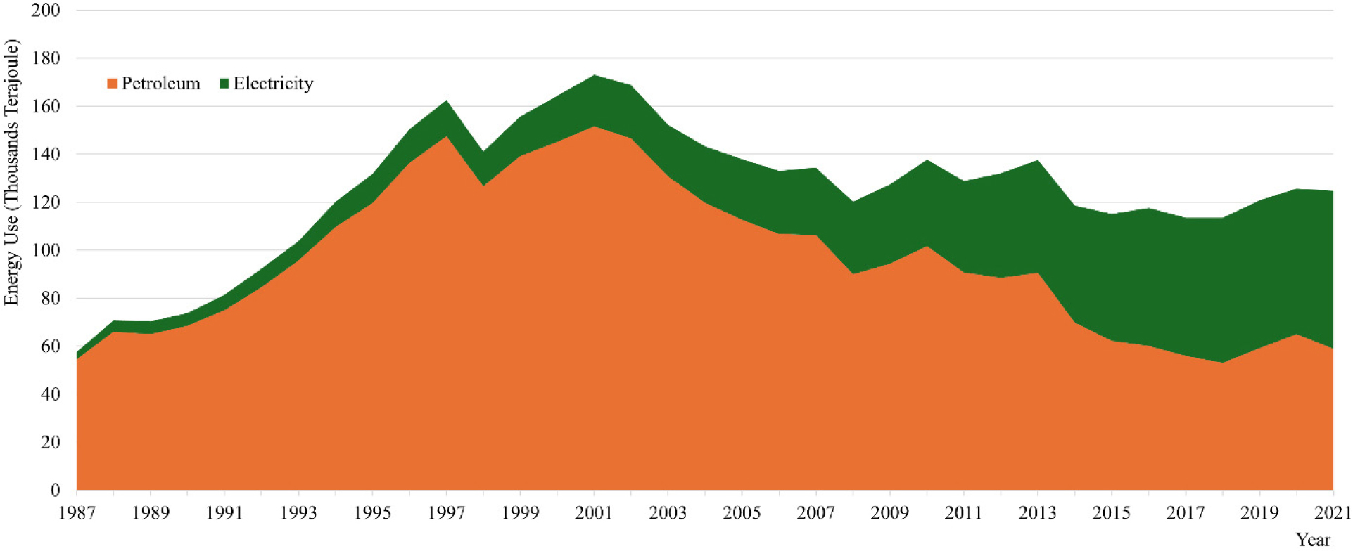
According to the Food and Agriculture Organization (FAO), the total amount of energy used for agricultural production is 124,822.5 thousand TJ in 2022, which has increased by 2.23% annually. Energy sources widely used in Korea are petroleum, electricity, and natural gas. Fig. 1 shows that the total amount of energy used has continuously decreased since 2001. Petroleum is a major energy source for agricultural production, which accounts for 80% and above from 1987 to 2005. However, electricity has become a dominant energy source recently, and its share of the total amount of energy use has been approximately 50% since 2017. Fig. 1 also suggests a change of energy sources from petroleum to electricity in food production because of its efficiency and versatility (Shih et al., 2018). For example, electric tractors and weeders are results of the electrification of agricultural applications, which switch power sources from fossil fuels to electricity (Fu and Niu, 2023).

https://cdn.apub.kr/journalsite/sites/ales/2024-036-04/N0250360411/images/ales_36_04_11_F1.jpg

Fig. 1.

Energy use in agricultural production in Korea.
Source: FAOSTAT

Technological progress has potential to maximize a benefit of limited resources such as water, energy, and space to meet the increasing food demand and supply (Hemathilake and Gunathilake, 2022). Technology gaps between countries are one of the major factors determining agricultural land use for food production, affecting food dependency on foreign countries (Villoria, 2019). Considering that agricultural land use is proportional to farm size, it will be commensurate with an amount of production inputs such as energy consumption in agricultural production. Moreover, advanced technology in farm equipment and machinery used in agricultural practices increases agricultural production efficiency, which makes farmers use energy sources efficiently, allowing them to use renewable energy sources by replacing conventional ones such as fossil fuels (Dimitrijević, 2023). It is also consistent with Bonny (1993), who states that agriculture consumes energy efficiently reducing the total amount of fossil fuel as a technical evolution of agriculture. Additionally, technological advancement is important for policymakers who should take production efficiency into account because it can reduce energy consumption without side effects of economic growth on the environment. (Hasanov and Mikayilov, 2021). The Korean government also has been working on several programs to promote energy conservation and efficient use (Kim et al., 2010). To make energy consumption efficient, it is necessary to introduce advanced agricultural technology such as fuel-efficiency equipment and machinery as well as environmental-friendly agricultural practices (Jeong et al., 2023).

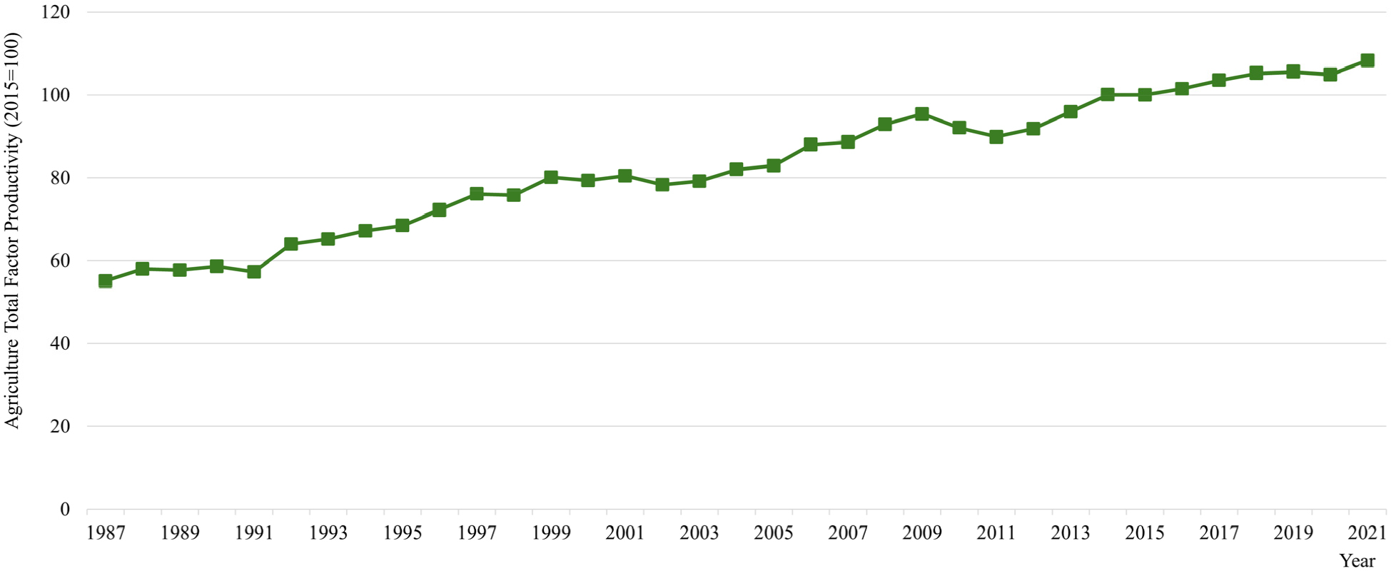
In this perspective, agricultural Total Factor Productivity (TFP) is one of the important factors affecting energy use in agricultural sectors, especially, the formation of energy demand (Hasanov and Mikayilov, 2021). It is different from crop yields or agricultural value added per production input because it measures the overall agricultural productivity concerning a broader set of production inputs (USDA ERS). It measures production technology and efficiency by comparing a ratio between total output and input used in food production (Fuglie et al., 2024). The growth of TFP is a result of changes in farm revenue and production costs by the weighted sum of them (USDA ERS). Fig. 2 shows agricultural TFP in Korea from1987 to 2021. Since 1987, agricultural TFP has increased by 1.95% annually, indicating that input uses may decrease relatively compared to agricultural output or vice versa. It implies that farmers have experienced an improvement in agricultural productivity by lowering a unit cost in input uses (Fuglie et al., 2024). There is some literature showing the relationship between energy consumption and TFP. Hasanov et al. (2019) states that energy consumption decreases as TFP is growing. Usman et al. (2021) emphasize that technological advancement such as an expansion of internet uses can positively contribute to economic growth with an achievement of energy efficiency. Shen et al. (2019) state that an increase in agricultural productivity through technological progress can lower energy usage related to farming practices.

https://cdn.apub.kr/journalsite/sites/ales/2024-036-04/N0250360411/images/ales_36_04_11_F2.jpg

Fig. 2.

Agricultural total factor productivity in Korea.
Source: USDA ERS, 2024

Energy consumption for agricultural production relates to the emissions of pollutants such as greenhouse gas (GHG) and other residues that adversely affect the environment (Agras and Chapman, 1999). Ultimately, energy efficiency by advanced agricultural production relates to improvements in the environment of a country directly. This is a view of a conservation hypothesis that economic growth influences energy consumption to confirm that energy policies pursuing higher efficiency in energy use can affect economic growth in a country (Alshehry and Belloumi, 2015). Additionally, Kuznets (1967) develops a hypothesis for the relationship between environmental degradation and economic growth, finding that environmental degradation is severe at the initial stage of economic development, but it is addressed at the later stage of economic development after a turning point. In turn, the Kuznets curve hypothesis implies that an increase in energy consumption is observed at the initial stage of economic growth, but energy consumption would decrease after the turning point and at the later stage of economic growth based on the assumption that environmental degradation is directly proportional to an increase in energy consumption in terms of a conservation hypothesis.

The objective of this study is to examine the existing literature about the relationship between technological progress and energy consumption controlling agricultural value-added and agricultural land use, applying the framework to Korean agricultural sectors. Agriculture in Korea is one of the good examples to investigate the relationship between energy consumption and technological progress. Firstly, energy sources for agricultural production are heavily dependent on foreign countries in South Korea because of insufficient natural resources. Secondly, Korean agriculture has been vulnerable to the international market because of Free Trade Agreements that have been implemented since 2003 with various government support programs that keep agricultural sectors competitive. Both facts indicate that although restrictions on energy demand and supply for agricultural production obstruct agricultural development and threaten food security, improvement in agricultural productivity is a key issue in a reduction in energy-related input costs in Korean agricultural sectors (Jeong et al., 2023).

Secondly, we will construct a quadratic term of agricultural value-added for assessing the Kuznets curve hypothesis for agricultural energy consumption and agricultural value-added. To the best of our knowledge, it is the first attempt that estimates the long-run relationship between energy consumption and agricultural productivity and examines the Kuznets curve hypothesis for energy consumption and growth in agricultural sectors based on the input-demand function framework.

Material and Methods

Data

To confirm the relationship between energy consumption and technological progress in agricultural sectors and a Kuznets curve hypothesis between energy consumption and growth in agriculture, we construct the following equation suggested by Hasanov et al. (2019).

(1)

A G E C_{t} = β_{0} + β_{1} A G T F P_{t} + β_{2} A G Y_{t} + β_{3} A G Y_{t}^{2} + β_{0} A G L A N D_{t} + e_{t}

where, $A G E C_{t}$ is the gross amount of energy consumption in agricultural sectors provided by FAO STAT. $A G T F P_{t}$ is agricultural factor productivity as a proxy for technological progress in agricultural sectors. Agricultural factor productivity is sourced from the United States Department of Agriculture Economic Research Service (USDA ERS) and is estimated by Fuglie et al. (2024). $A G Y_{t}$ and $A G Y_{t}^{2}$ are agricultural value-added (Real Prices, Constant 2014-2016 U.S. Dollar) and its quadratic term, respectively. $A G L A N D_{t}$ is arable land. Agricultural value-added and arable land are sourced from FAO STAT. This study uses annual (time-series) data for Korea from 1987 to 2021. The study period was chosen based on the data availability for all-time series data. Descriptive statistics are presented in Table 1.

Table 1.

Descriptive statistics

Variables	Unit	Mean	Std. dev.	Min	Max
$A G E C_{t}$	Terajoule	124,620.88	28,815.90	57,656.56	174,048.93
$A G T F P_{t}$	2015=100	82.91	16.14	55.1	108.26
$A G Y_{t}$	Million Dollar	43,444.76	3,750.07	34,826.85	50,184.97
$A G L A N D_{t}$	1,000 ha	1,648.41	199.39	1,343.00	2,007.00

Note: Std. dev. indicates standard deviation. Agricultural value-added ( $A G Y$ ) is a real value (constant 2014-2016 US dollar).

Methodology

This study applies an empirical analysis through an Autoregressive Distributed Lag (ARDL) model with a cointegration test to estimate short- and long-run relationships between energy use and technological progress in agricultural sectors (Pesaran and Shin, 1999). Additionally, we also use the ARDL approach to confirm a Kuznets curve hypothesis between energy use and the growth of agricultural production. The ARDL model with a cointegration test has an advantage over other types of approaches because it is robust and efficient for a small sample size of time-series data (Latif et al., 2015). An endogeneity problem is also mitigated in the ARDL approach because of a free of residual correlation (Nkoro and Uko, 2016). Finally, an Error Correction Term (ECT) can be extracted from an ARDL model via a linear transformation with an integration of short-run adjustments with a long-run equilibrium (Nkoro and Uko, 2016).

The first step of an ARDL approach is to perform Unit Root (UR) tests for time series data. This is because the ARDL approach is applicable if time-series data are stationary at level (I(0)) or at first difference (I(1)) or a mixture of I(0) and I(1). We will use two types of unit root tests, Augmented Dicky-Fuller (ADF) (Dickey and Fuller, 1981) and Phillips-Perron (PP) (Phillips and Perron, 1988) tests. The ADF test is a method broadly utilized to confirm the stationarity of time-series data. A problem the ADF test has is that it does not properly work to deal with moving average errors, which may exist in time-series data (DeJong et al., 1992; Phillips and Perron, 1988; Schwert, 1987). Thus, we also perform the Phillips-Perron test for the robustness check of the ADF test because it is commonly used as an alternative to the ADF test (Arltová and Fedorová, 2016).

We can express the ARDL model using equation (1) as follows:

(2)

\begin{aligned} Δ A G E C_{t} = & β_{0} + \sum_{i = 1}^{p} γ_{i} Δ A G E C_{t - i} + \sum_{i = 0}^{q_{1}} δ_{i}^{1} A G T F P_{t - i} + \sum_{i = 0}^{q_{2}} δ_{i}^{2} A G Y_{t - i} + \sum_{i = 0}^{q_{3}} δ_{i}^{3} A G Y_{t - i}^{2} + \sum_{i = 0}^{q_{4}} δ_{i}^{4} A G L A N D_{t - i} + λ_{1} A G E C_{t - 1} + λ_{2} A G T F P_{t - 1} + λ_{3} A G Y_{t - 1} + λ_{4} A G Y_{t - 1}^{2} + λ_{5} A G L A N D_{t - 1} + η_{t} \end{aligned}

where, $β_{0}$ and $η_{t}$ are intercept and stochastic error terms, respectively. 𝛾 and 𝛿 ’s represent the short-run dynamics of the ARDL model, while 𝜆’s denote corresponds to the long-run relationship among variables. $p$ and $q$ ’s are an optimal lag length of variables selected by the Bayesian Information Criteria (BIC).

We will estimate equation (2) using a linear regression through an Ordinary Least Square (OLS) estimator. Then, we will use an ARDL bounds test to confirm the existence of the long-run relationship between variables. The null hypothesis of the ARDL bounds test (F-test) is $H_{0} : λ_{1} = λ_{2} = λ_{3} = λ_{4} = λ_{5} = 0$ and the alternative hypothesis is that at least one of 𝜆’s is not zero. The F-statistics calculated by the ARDL bounds test will be tested by I(0) and I(1) bounds (critical values) provided by Pesaran et al. (2001). If F-statistics value is greater than the I(1) bounds (and t-statistics value is less than the I(1) bounds), then we can reject the null hypothesis and conclude that there is a long-run relationship among variables.

We will transform from equation (2) to equation (3) by adding an Error Correction Term (ECT) to the ARDL model.

(3)

\begin{aligned} Δ A G E C_{t} = & β_{0} + \sum_{i = 1}^{p} γ_{i} Δ A G E C_{t - i} + \sum_{i = 0}^{q_{1}} δ_{i}^{1} A G T F P_{t - i} + \sum_{i = 0}^{q_{i}} δ_{i}^{2} A G Y_{t - i} + \sum_{i = 0}^{q_{3}} δ_{i}^{3} A G Y_{t - i}^{2} + \sum_{i = 0}^{q_{4}} δ_{i}^{4} A G L A N D_{t - i} + α E C T_{t - 1} + η_{t} \end{aligned}

where, $E C T_{t - 1}$ represents an error correction term and 𝛼 is the speed of adjustment coefficient towards a long-run equilibrium. A coefficient for the ECT associated with the long-run relationship should be negative and statistically significant to ensure that the shock in the short-run in the ARDL model will be convergent towards the long-run equilibrium (Narayan and Smyth, 2006). We also perform several diagnostic tests such as Breusch-Pagan (BP) test for detecting heteroskedasticity, Ramsey’s Regression Equation Specification Error Test (Ramsey’s RESET) for a functional form, Durbin-Watson (DW) d-statistics for autocorrelation in the residuals and Jarque-Bera (JB) test for normality of residuals to confirm ARDL model’s efficiency and consistency. Additionally, we will plot cumulative sum (CUSUM) and cumulative sum of squares (CUSUMSQ) charts to ensure the stability of the results of the ARDL model (Brown et al., 1975).

Results and Discussion

Table 2 presents the results of ADF and PP unit root tests on variables used in this study. Both ADF and PP tests show the time-series data are stationary at first difference level (I(1)), meaning that the ARDL model is applicable to this study.

Table 2.

Results of unit root tests

Variables	ADF				PP
	Level		1st Difference		Level		1st Difference
	No Trend	Trend	No Trend	Trend	No Trend	Trend	No Trend	Trend
$A G E C_{t}$	-2.32	-1.92	-4.72***	-5.15***	-3.41**	-2.55	-4.72***	-5.15***
$A G T F P_{t}$	-0.59	-2.92	-6.12***	-6.01***	-0.73	-3.03	-6.12***	-6.01***
$A G Y_{t}$	-1.81	-1.58	-6.49***	-6.45***	-2.65*	-2.28	-6.49***	-6.45***
$A G Y_{t}^{2}$	-1.84	-1.62	-6.37***	-6.34***	-2.53	-2.20	-6.37***	-6.34***
$A G L A N D_{t}$	-1.40	-2.44	-4.60***	-4.72***	-1.19	-1.92	-4.60***	-4.72***

Note: ***, **, and * indicate the 1%, 5%, and 10% significant levels, respectively. The null hypothesis for ADF and PP unit root tests is that time series have a unit root.

For the ARDL model with a cointegration test using ARDL bounds test, the optimal lag lengths of variables are determined by BIC with the maximum lag lengths of up to 4 to avoid the collinearity of the ARDL model. The optimal lag lengths of variables selected by BIC are 2, 4, 4, 1, 2 for energy consumption in agricultural sectors ( $p$ ), agricultural total factor productivity ( $q_{1}$ ), agricultural value-added ( $q_{2}$ ), the quadratic term of agricultural value-added ( $q_{3}$ ), and arable land ( $q_{4}$ ), respectively. Table 3 presents the results of the ARDL bounds test for the long-run relationship. The number of F-statistics (t-statistics) for the ARDL model is much greater (smaller) than the I(1) critical values. Thus, the results imply that we can reject the null hypothesis and conclude that there exists a long-run relationship among variables in the ARDL model.

Table 3.

Results of bounds test for cointegration relationship

Test-Statistics		1% Critical Value
Test-Statistics		I(0) bounds	I(1) bounds
F-statistics	19.384	3.74	5.06
t-statistics	-8.351	-3.43	-4.60

Note: The null hypothesis for bounds test is that the cointegration relationship does not exist among variables. The null hypothesis is rejected if the value of F-statistics is greater than I(1) bounds (5.06) and if that of t-statistics is smaller than the I(1) bounds (-4.60).

Table 4 provides the results of the ARDL model for long- and short-run relationships among variables. The results confirm that the ECT is -1.752 and statistically significant at the 1% level, implying that a short-run shock will converge towards a long-run equilibrium in a dampening manner (Kim and Seok, 2021; Narayan and Smyth, 2006).

Table 4.

Estimation results for the long- and short-run

ARDL (2, 4, 4, 1, 2)		Estimates	t-statistics
Long-run	$A G T F P_{t}$	-0.021 (0.005)***	-3.99
	$A G Y_{t}$	0.429 (0.048)***	8.88
	$A G Y_{t}^{2}$	-0.004 (0.001)***	-7.65
	$A G L A N D_{t}$	-0.002 (0.000)***	-3.39
Short-run	$Δ \ln A G E C_{t - 1}$	0.771 (0.167)***	4.62
	$Δ A G T F P_{t}$	0.007 (0.010)	0.71
	$Δ A G T F P_{t - 1}$	-0.018 (0.009)*	-2.12
	$Δ A G T F P_{t - 2}$	-0.022 (0.006)***	-3.95
	$Δ A G T F P_{t - 3}$	-0.008 (0.005)	-1.75
	$Δ A G T_{t}$	-0.396 (0.100)***	-3.96
	$Δ A G T_{t - 1}$	-0.008 (0.008)	-1.09
	$Δ A G T_{t - 2}$	0.023 (0.005)***	4.70
	$Δ A G Y_{t - 3}$	0.015 (0.006)**	2.63
	$Δ A G Y_{t}^{2}$	0.004 (0.001)***	3.78
	$Δ A G L A N D_{t}$	0.003 (0.001)***	3.99
	$Δ A G L A N D_{t - 1}$	0.002 (0.001)**	2.74
Constant		9.590 (3.801)**	2.52
$E C T_{t - 1}$		-1.752 (0.210)***	-8.35
Diagnostic test		statistics	p-value
Heteroskedasticity (BP test)		1.09	0.297
Functional Form (RESET test)		0.37	0.774
Jarque-Bera Normality Test		0.870	0.647
Durbin Watson d-statistic (18, 31)		2.135
$R^{2}$		0.944
$N$		31

Note: ***, **, and * indicate the 1%, 5%, and 10% significant levels, respectively. Standard errors are the numbers in parentheses.

The results show that an increase in agricultural TFP leads to a decrease the agricultural energy consumption by 0.021% on average in the long-run. It is consistent with the results by Hasanov et al. (2019) who state that TFP is a component of a production function, affecting efficiency gains from technological advancements through Research and Development (R&D) and institutional improvement. Additionally, energy intensity will be improved through an increase in technological progress, which means the same amount of output using less input or the same amount of input producing more output. In the short-run, the estimates of agricultural TFP tend to be insignificant because of technological progress (Hailu, 2023).

The positive sign of the long-run coefficient of agricultural value-added and the negative sign of its quadratic term show an inverted U-shape relationship between energy consumption and agricultural economic development, meaning that the Kuznets curve hypothesis holds. It suggests energy consumption increases at the initial stage of agricultural development, but it eventually decreases later due to the maturity of agricultural production. It is consistent with the results of Bonny (1993) who states that an increase in energy consumption is observed to produce a given amount of agricultural product with efficient use of energy in agricultural sectors. It also implies that the degree of environmental contamination related to energy consumption may increase at the initial stage of agricultural economic development, but it may decrease at the later stage of development in terms of the research by Kuznets (1967). However, in the short-run, Kuznets curve hypothesis does not hold because signs of the linear terms of agricultural value-added with time lags are inconsistent.

An expansion in arable land is also related to a decrease in energy consumption in agricultural sectors. Although the amount of energy used for agricultural production tends to increase as a response to an expansion of arable land, the negative coefficient of arable land reflects a decreasing trend of arable land in the long-run. In other words, a decreasing trend of arable land for agricultural production and an increasing trend in energy consumption for food production may result in a negative relationship between them in the long-run. Unlike the long-run relationship between energy consumption and arable land, the estimates of arable land in the short-run have positive signs, which means that an increase in energy consumption is expected as an expansion of arable land.

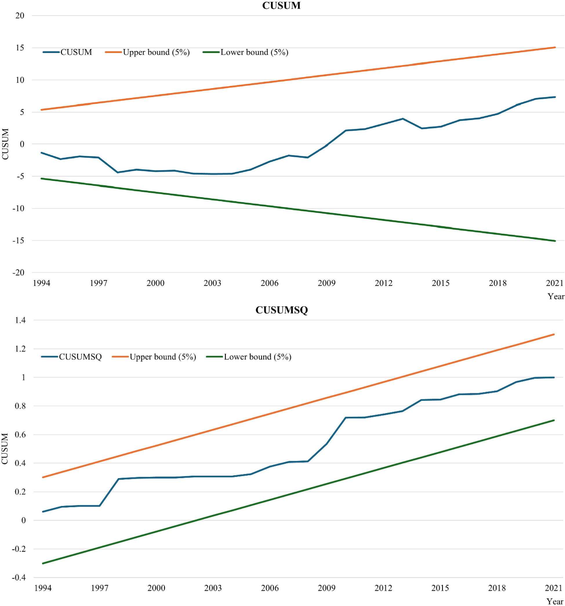
Finally, the results of diagnostic tests suggest that the ARDL model used in this study does not have problems. The result of the BP test shows that the variance of the residuals of the ARDL model does not suffer from a heterogeneity problem. The RESET test also indicates that the model specification does not have a problem in the estimation. Jarque-Bera Normality test and Durbin-Watson d-statistics suggest that the distribution of the residuals is normal and the ARDL model does not have a serial autocorrelation. Fig. 3 shows CUSUM and CUSUM Square charts for the stability of the ARDL results for the short- and long-run model. We can confirm that CUSUM and CUSUMSQ of the ARDL model are within the critical bounds of 5% of significant levels.

https://cdn.apub.kr/journalsite/sites/ales/2024-036-04/N0250360411/images/ales_36_04_11_F3.jpg

Fig. 3.

CUSUM and CUSUM Square (CUSUMSQ) charts for ARDL model.

Conclusion

This study examines the short- and long-run relationship between technological progress and energy consumption in agricultural sectors through an ARDL model. To represent technological progress in agricultural production, we utilize agricultural TFP, which is a ratio between agricultural output and input. We also investigate a framework between agricultural value-added and energy consumption through a Kuznets Curve hypothesis to estimate the shape of a relationship between the amount of energy used and growth in agricultural sectors.

Our results from the ARDL in the long-run suggest that enhancement of agricultural productivity by technological progress is beneficial for energy use in food production. The Kuznets curve hypothesis is also confirmed because the coefficient of agricultural value-added is positive and its quadratic term is negative, meaning that energy consumption increases at the initial stage of agricultural development, but decreases at the later stage of it. Moreover, while energy consumption is commensurate with an expansion of arable land in the short-run, it is inversely proportional to arable land due to a decreasing tend of it in the long-run.

Our empirical analysis suggests several contributions to the literature and policy implications. First, government support programs for agricultural technology development should be developed because they are beneficial for farmers by enhancing the efficiency of agricultural production. Especially, they educate younger farmers who may tend to introduce newly developed technologies and agricultural practices It is a good opportunity for farmers to improve their profitability by lowering production costs with an advanced energy efficiency. Second, growth in agriculture will make the environment better due to lowering input use such as petroleum and electricity. Additionally, electricity, which is generally more efficient than other conventional energy sources, is replacing petroleum products and alleviating environmental concerns.

This study also has a limitation on an analysis that cannot explain more details on the impacts of technological progress in energy consumption by a variety of sources. In other words, we are dealing with energy sources petroleum, electricity, and natural gas, while there are different sources, such as renewable energy (e.g., solar, wind, hydro, and biomass). We can also measure how renewable energy sources can replace conventional ones and how agricultural technological progress makes them different in agricultural production. Based on the results of this study, we can conduct future research on the causal relationship among agricultural technological progress, the replacement between conventional energy sources and renewable ones, and the impacts of them on the environment including emissions of greenhouse gases, carbon dioxide, nitrogen oxide, and methane. Using a dynamic analysis of causal inferences, future research will contribute to the literature on the environmental impacts of advancement in agricultural sectors in South Korea.

References

Agras, J., Chapman, D. (1999) A dynamic approach to the Environmental Kuznets Curve hypothesis. Eco Econ 28:267-277.

10.1016/S0921-8009(98)00040-8

Alshehry, A. S., Belloumi, M. (2015) Energy consumption, carbon dioxide emissions and economic growth: The case of Saudi Arabia. Renew Sus Energ Rev 41:237-247.

10.1016/j.rser.2014.08.004

Arltová, M., Fedorová, D. (2016) Selection of Unit Root Test on the Basis of Length of the Time Series and Value of AR(1) Parameter. Statistika 96:47-64.

Bonny, S. (1993) Is agriculture using more and more energy? A French case study. Agr Syst 43:51-66.

10.1016/0308-521X(93)90092-G

Brown, R. L., Durbin, J., Evans, J. M. (1975) Techniques for Testing the Constancy of Regression Relationships over Time. J Roy Stat Soc B Met 37:149-192.

10.1111/j.2517-6161.1975.tb01532.x

DeJong, D. N., Nankervis, J. C., Savin, N. E., Whiteman, C. H. (1992) The power problems of unit root test in time series with autoregressive errors. J Econometrics 53:323-343.

10.1016/0304-4076(92)90090-E

Dickey, D. A., Fuller, W. A. (1981) Likelihood Ratio Statistics for Autoregressive Time Series with a Unit Root. Econometrica 49:1057-1072.

10.2307/1912517

Dimitrijević, M. S. (2023) Technological progress in the function of productivity and sustainability of agriculture: The case of innovative countries and the Republic of Serbia. J Agric Food Res 14:100856.

10.1016/j.jafr.2023.100856

Fu, X., Niu, H. (2023) Key technologies and applications of agricultural energy Internet for agricultural planting and fisheries industry. IPA 10:416-437.

10.1016/j.inpa.2022.10.004

Fuglie, K. O., Morgan, S., Jelliffe, J. (2024) World agricultural production, resource use, and productivity, 1961-2020. Report No. EIB-268. USDA ERS,

10.32747/2024.8327789.ers

Hailu, G. (2023) Reflections on technological progress in the agri-food industry: Past, present, and future. Can J Agr Econ 71:119-141.

10.1111/cjag.12325

Hasanov, F. J., Liddle, B., Mikayilov, J. I., Bollino, C. A. (2019) How Total Factor Productivity Drives Long-Run Energy Consumption in Saudi Arabia. pp.195-220. In M. Shahbaz and D. Balsalobre, eds. Energy and Environmental Strategies in the Era of Globalization. Green Energy Technol.

10.1007/978-3-030-06001-5_8

Hasanov, F. J., Mikayilov, J. I. (2021) The impact of total factor productivity on energy consumption: Theoretical framework and empirical validation. Energy Strategy Reviews 38:100777.

10.1016/j.esr.2021.100777

Hemathilake, D. M. K. S., Gunathilake D. M. C. C. (2022) Chapter 31 - Agricultural productivity and food supply to meet increased demands. pp.539-553. In R. Bhat, ed. Future Foods.

10.1016/B978-0-323-91001-9.00016-5

IPCC (2023) Summary for Policymakers. In: Climate Change 2023: Synthesis Report. Contribution of Working Groups I, II and III to the Sixth Assessment Report of the Intergovernmental Panel on Climate Change, IPCC.

Jeong, H., Sung, J., Lim, Y. Lim, J. H., Im, J., Lee, S. (2023) A Study on Vitalizing Green Economy in the Agricultural and Forestry Sectors (Year 2 of 3). R958. Korea Rural Economic Institute.

Kim, S. E., Seok, J. H. (2021) Trade openness and horizontal agricultural income inequality in Korea: focusing on sectoral income differences. J Asia Pac Econ 28(4):1580-1600.

10.1080/13547860.2021.1991087

Kim, Y. J., Park, K. H., Kang, C. Y., Kim. Y. H., Kim, H. H., Oh, S. I. (2010) Structure and Prospect for Supply and Demand of Energy in Agricultural Sector, R614-1, Korea Rural Economic Institute.

Kuznets, S. (1967) Modern Economic Growth: Rate, Structure, and Spread. New Haven and London. Yale University Press.

Latif, N. W. A., Abdullah, Z., Razdi, M. A. M. (2015) An Autoregressive Distributed Lag (ardl) Analysis of the Nexus Between Savings and Investment in the Three Asian Economies. JDA 49:323-334.

10.1353/jda.2015.0154

Majeed, Y., Khan, M. U., Waseem, M., Zahid, U., Mahmood, F., Majeed, F., Sultan, M., Raza, A. (2023) Renewable energy as an alternative source for energy management in agriculture. Energy Rep 10:344-359.

10.1016/j.egyr.2023.06.032

Narayan, P. K., Smyth, R. (2006) What Determines Migration Flows from Low-Income to High-Income Countries? An Empirical Investigation of Fiji-U.S. Migration 1972-2001. Contemp Econ Policy 24:332-342.

10.1093/cep/byj019

Nkoro, E., Uko, A. K. (2016) Autoregressive Distributed Lag (ARDL) cointegration technique: application and interpretation. Journal of Statistical and Econometric Methods 5:1-3.

Omer, A. M. (2008) Energy, environment and sustainable development. Renew Sust Energ Rev 12:2265-2300.

10.1016/j.rser.2007.05.001

Park, J., Kim, Y. (2019) The Effects of Renewable Energy in Agricultural Sector. JKAIS 20:224-235.

Pesaran, M. H., Shin, Y. (1999) An Autoregressive Distributed-Lag Modelling Approach to Cointegration Analysis. pp.371-413. In S. Strøm, ed. Econometrics and Economic Theory in the 20th Century: The Ragnar Frisch Centennial Symposium. Econom Soc Monogr. Cambridge: Cambridge University Press.

10.1017/CCOL521633230.011

Pesaran, M. H., Shin, Y., Smith, R. J. (2001) Bounds Testing Approaches to the Analysis of Level Relationships. J Appl Econom 16:289-326.

10.1002/jae.616

Phillips, P. C. B., Perron, P. (1988) Testing for a Unit Root in Time Series Regression. Biometrika 75:335-346.

10.1093/biomet/75.2.335

Schwert, G. W. (1987) Effects of model specification on tests for unit roots in macroeconomic data. J Monetary Econ 20:73-103.

10.1016/0304-3932(87)90059-6

Shen, N., Liao, H., Deng, R., Wang, Q. (2019) Different types of environmental regulations and the heterogeneous influence on the environmental total factor productivity: Empirical analysis of China's industry. J Clean Prod 211:171-184.

10.1016/j.jclepro.2018.11.170

Shih, C. F., Zhang, T., Li, J., Bai, C. (2018) Powering the Future with Liquid Sunshine. Joule 2:1925-1949.

10.1016/j.joule.2018.08.016

USDA ERS (2024) International Agricultural Productivity data product. Available at: https://www.ers.usda.gov/data-products/international-agricultural-productivity/documentation-and-methods/

Usman, A., Ozturk, I., Hassan, A., Maria Zafar, S., Ullah, S. (2021) The effect of ICT on energy consumption and economic growth in South Asian economies: An empirical analysis. Telemat Inform 58:101537.

10.1016/j.tele.2020.101537

Villoria, N. B. (2019) Technology Spillovers and Land Use Change: Empirical Evidence from Global Agriculture. Am J Agr Econ 101:870-893.

10.1093/ajae/aay088

Woods, J., Williams, A., Hughes, J. K., Black, M., Murphy, R. (2010) Energy and the food system. Philos T R Soc B 365:2991-3006.

10.1098/rstb.2010.017220713398PMC2935130

Journal of Agricultural, Life and Environmental Sciences ISSN:2233-8322(Print) 2508-870X(Online)

Preview

Evaluating Technological Progress and Energy Consumption in Korean Agricultural Sectors: An Application of the Autoregressive Distributed Lag Model Approach

ABSTRACT

MAIN

Fig. 1.

Energy use in agricultural production in Korea.Source: FAOSTAT

Fig. 2.

Agricultural total factor productivity in Korea.Source: USDA ERS, 2024

(1)

Table 1.

Descriptive statistics

(2)

(3)

Table 2.

Results of unit root tests

Table 3.

Results of bounds test for cointegration relationship

Table 4.

Estimation results for the long- and short-run

Fig. 3.

CUSUM and CUSUM Square (CUSUMSQ) charts for ARDL model.

References

Energy use in agricultural production in Korea.
Source: FAOSTAT

Agricultural total factor productivity in Korea.
Source: USDA ERS, 2024