


Introduction
Materials and Methods
Study area
Data collection and preprocessing
Transformer-based Sequence-to-Sequence Model for Multi-step Chl-a Forecasting
Model Setup for Chl-a Forecasting
Evaluation Metrics
Results and Discussion
Comparison of Chl-a Forecasting Performance Across Different Lookback Windows
Interpretation of Forecasting Mechanism based on Cross-Attention
Conclusion
Introduction
The risk of algal blooms in agricultural reservoirs has increased substantially in recent years owing to the combined effects of climate change and elevated nutrient loading from surrounding watersheds (Jargal et al., 2021; Zahir et al., 2025; Zhang et al., 2025). These lentic systems are particularly susceptible to rapid increases in chlorophyll-a (Chl-a) concentration when elevated water temperatures coincide with nutrient-rich runoff following rainfall events. In addition, the water quality in such reservoirs exhibits pronounced temporal variability and can fluctuate at subdaily to hourly scales. Under these conditions, conventional management strategies based on postobservational data are insufficient for timely and effective interventions. Accordingly, there is a growing need for proactive water quality forecasting systems that can support real-time decision-making (Guan et al., 2022; Rozemeijer et al., 2025).
In response to this need, deep-learning approaches have been increasingly adopted in order to model complex and nonlinear temporal patterns in water quality time series. Among these approaches, Transformer-based Sequence-to-Sequence (S2S) architectures have demonstrated notable advantages in multi-step forecasting tasks owing to their self-attention mechanisms, which enable the capture of long-range dependencies without relying on recurrence (Wen et al., 2023; Zhou et al., 2021). Despite these advancements, a substantial portion of existing studies have focused primarily on performance comparisons among different model architectures. In contrast, relatively limited attention has been paid to the optimization of key input configurations. In particular, the selection of a lookback window, defined as the length of historical input data used for forecasting, is often determined empirically or fixed without rigorous optimization across different applications.
Agricultural reservoirs exhibit heterogeneous hydrological responses and pollutant transport processes that are influenced by site-specific characteristics such as reservoir size, inflow dynamics, and watershed conditions (Bieroza et al., 2020; Jo et al., 2021). These factors govern both the lag time and cumulative effects of nutrient inputs, indicating that the optimal lookback window should vary depending on the environmental context. A lookback window that is too short may fail to capture essential temporal patterns such as diurnal cycles. Conversely, an excessively long window may introduce redundant or irrelevant information, which can act as noise during model training and degrade the forecasting performance. Despite these implications, systematic investigations into the influence of lookback window length on both forecasting accuracy and model interpretability in multivariate environmental systems remain limited.
Therefore, the objective of this study was to develop a Transformer-based S2S model for 72 h ahead forecasting of Chl-a in an agricultural reservoir and to identify the optimal lookback window that ensured robust and stable forecasting performance. In order to achieve this objective, multiple lookback window scenarios were constructed, and their performances were systematically evaluated across different forecasting horizons. By quantitatively evaluating the trade-off between information gain and noise introduction, this study not only advances the understanding of the relationship between input configurations and model reliability but also provides a systematic framework that can contribute to the development of more accurate and practical data-driven models for reservoir water quality forecasting.
Materials and Methods
Study area
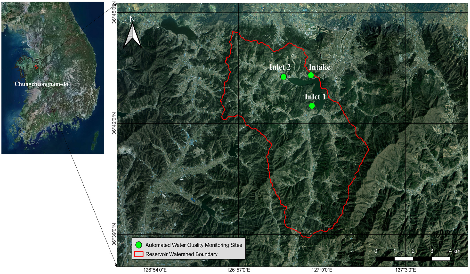
This study was conducted in Gungpyeong Reservoir, an agricultural reservoir located in Donghwa-ri, Songak-myeon, Asan-si, Chungcheongnam-do, Republic of Korea (Fig. 1). The reservoir provides irrigation water to a command area of 1,108.0 ha and is characterized by a total watershed area of 4,333 ha and an effective storage capacity of 6,717.0 × 103 m3. A monitoring network was established within the reservoir to support water quality management. Periodic water quality surveys are conducted approximately four-seven times per year. In addition, automatic monitoring stations were installed at two inflow points and one intake point, enabling continuous measurements at 10-minute intervals. This system enables the acquisition of high-resolution time-series water quality data.
In recent years, the Gungpyeong Reservoir has exhibited increasing variability in water quality conditions. During summer, elevated water temperatures combined with nutrient availability increase the likelihood of algal bloom development and subsequent hypoxic conditions. These processes can lead to the deterioration of water quality and also ecological disturbance. Notably, fish kill events were reported in the summers of 2021 and 2023, highlighting the need for the proactive forecasting of water quality dynamics and the development of systematic management strategies.
Data collection and preprocessing
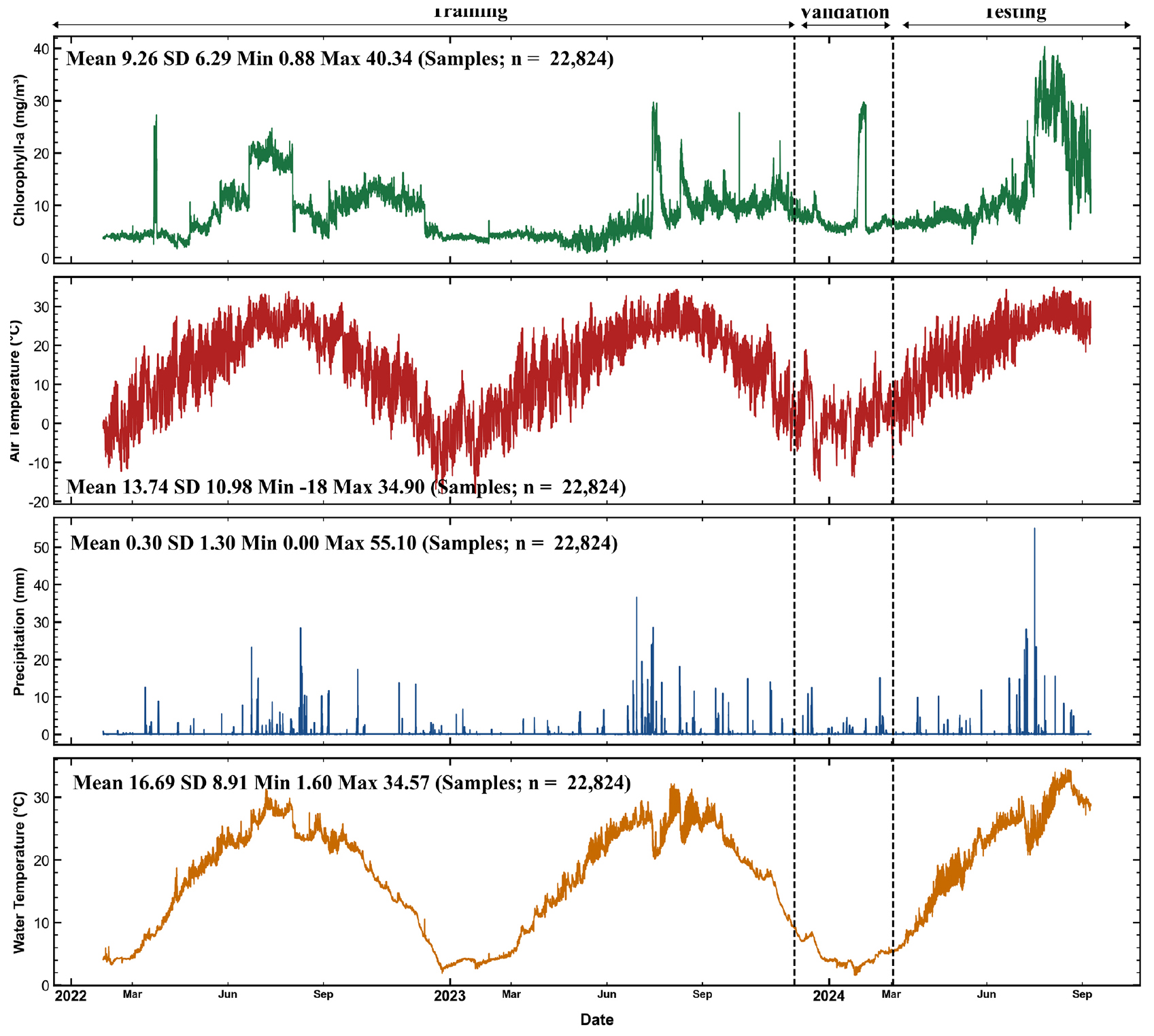
High-resolution water quality data were collected from an automatic monitoring station installed at the intake point of Gungpyeong Reservoir. The dataset spans from January 1, 2022, to September 11, 2024, and was originally recorded at 10-minute intervals. For time-series analysis, raw observations were aggregated into hourly mean values. The meteorological data corresponding to the same period were also incorporated. Specifically, the hourly air temperature (Tair, °C) and precipitation (PCP, mm/h) were obtained from the Cheonan Automated Synoptic Observing System. These data were temporally aligned with water quality observations to construct a multivariate time series dataset. The target variable in this study was chlorophyll-a concentration (Chl-a, mg/m3). The input variables included Tair, PCP, water temperature (Twater, °C), and historical Chl-a. Prior to model development, all of the variables were standardized to improve the numerical stability and convergence during training. Standardization was performed using StandardScaler, which was fitted to the training portion of the dataset and subsequently applied to the entire dataset. The dataset was chronologically divided into training (70%), validation (10%), and testing (20%) subsets to preserve temporal dependency and prevent data leakage (Fig. 2).
Transformer-based Sequence-to-Sequence Model for Multi-step Chl-a Forecasting
A Transformer is a neural network architecture based on a self-attention mechanism that captures dependencies across different time steps within a sequence (Vaswani et al., 2017). Unlike recurrent neural network-based models, the Transformer processes sequence data in parallel, thus enabling efficient modeling of long-range dependencies and complex temporal patterns in time-series data. In this study, an autoregressive (AR) sequence-to-sequence model based on the Transformer encoder-decoder architecture was developed for the multi-step forecasting of Chl-a. The overall architecture is illustrated in Fig. 3.
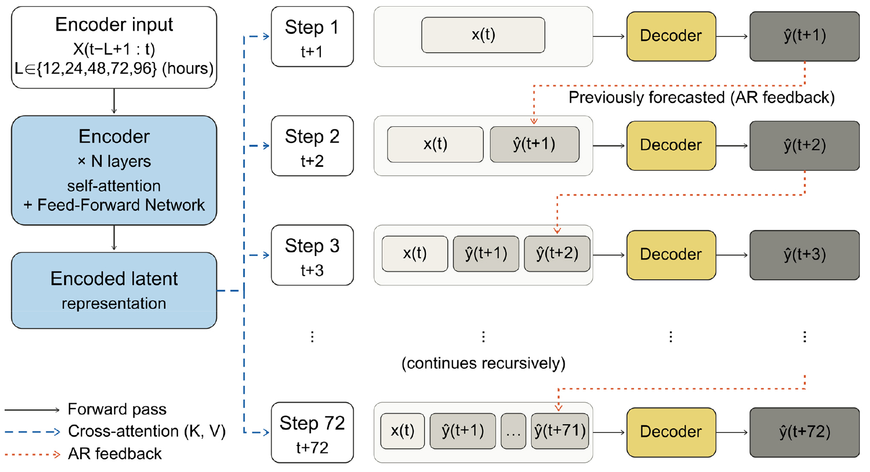
Because the Transformer does not inherently encode the sequential order, sinusoidal positional encoding was added to the input embeddings to preserve the chronological structure of the sequence. The encoder receives a multivariate lookback sequence X(t-L+1:t) = [x(t-L+1), …, x(t)], where each x(t) = [Chl-a(t), Tair(t), PCP(t), Twater(t)] is the observation vector at time t, and L is the lookback window length (L∈{12, 24, 48, 72, 96} hours). Through stacked layers of multihead self-attention and positionwise feed-forward networks with residual connections and layer normalization, the encoder learns latent representations that capture nonlinear relationships and intervariable dependencies. Because the lookback sequence is fixed during forecasting, the encoder is executed only once, and its output is shared across all decoding steps via cross attention.
The decoder generates 72 h forecasts autoregressively. In the first decoding step (k = 1), the decoder is initialized using the most recent observation vector, x(t). At each subsequent step k, the decoder input is extended with previously forecasted values, and masked self-attention ensures that each forecast depends only on earlier time steps, thereby preserving causality. Cross-attention allows the decoder to selectively attend to relevant time steps from the encoder output and dynamically identify influential historical patterns for each forecasting step.
Although the decoder produces forecasts for all of the four variables at every step, only the forecasted Chl-a, denoted ŷ(t+k) for k = 1, 2, …, 72, is retained as the final forecasting output. For AR feedback, the forecasted Chl-a and Twater were recursively fed back as inputs for the next decoding step, whereas Tair and PCP were replaced with their observed values at the forecasting horizon, representing the use of external weather forecasts available in real-world operational settings. Finally, the forecasted Chl-a values were inverse-transformed to their original scales (mg/m3) for evaluation. In order to enhance interpretability, cross-attention weights from the decoder were extracted and analyzed to quantify the relative importance of the historical time steps in the forecasting process.
Model Setup for Chl-a Forecasting
In this study, five distinct scenarios were constructed with input sequence lengths of 12, 24, 48, 72, and 96 h to quantitatively identify the impact of the historical observation reference period on the long-term multi-step forecasting performance. The Optuna framework (Akiba et al., 2019) was used to derive the optimal model architecture for each scenario. The search space for each hyperparameter is listed in Table 1. To ensure an objective comparison of the forecasting performance across scenarios, the batch size and maximum number of training epochs were fixed at 128 and 150, respectively.
Because the number of available training samples varies depending on the lookback window length, direct chronological splitting can lead to inconsistencies in the validation and test periods across scenarios. To address this issue, the validation and test target periods were aligned based on the maximum lookback setting. For each lookback scenario, the starting indices of the validation and test samples were adjusted so that all models generated forecasts over the same unseen future periods.
The model performance was evaluated by analyzing the changes in forecasting accuracy according to lead time, reflecting the characteristics of multi-step forecasting. The overall forecasting stability among the scenarios was assessed by calculating the average performance across the entire forecasting horizon from 1 to 72 h. In addition, a scatter plot analysis was performed to examine the relationship between the forecasted and observed values.
Table 1.
Hyperparameter Search Space Used in Optuna-Based Optimization
Evaluation Metrics
The Nash-Sutcliffe Efficiency (NSE) (Nash and Sutcliffe, 1970) and Root Mean Square Error (RMSE) were employed as evaluation metrics. The NSE represents the variance of the model forecasting error relative to the variance of the observed values. This metric ranges from - to 1, where a value closer to 1 indicates superior forecasting performance. RMSE represents the absolute magnitude of the error between the forecasted and observed values, with lower values indicating higher forecasting accuracy.
Results and Discussion
Comparison of Chl-a Forecasting Performance Across Different Lookback Windows
The optimal hyperparameters for each lookback window scenario are presented in Table 2. The forecasting performance was evaluated based on the models constructed under these optimized conditions. The NSE and RMSE values at each forecasting horizon for the Transformer-based S2S model with varying lookback window lengths are shown in Fig. 4 and Table 3. Overall, a consistent decline in performance was observed across all scenarios as the forecasting horizon increased (Fig. 4), which was attributed to error accumulation in the multi-step forecasting process (Bontempi et al., 2012).
Table 2.
Optimal hyperparameters for each lookback window scenario derived through the Optuna framework
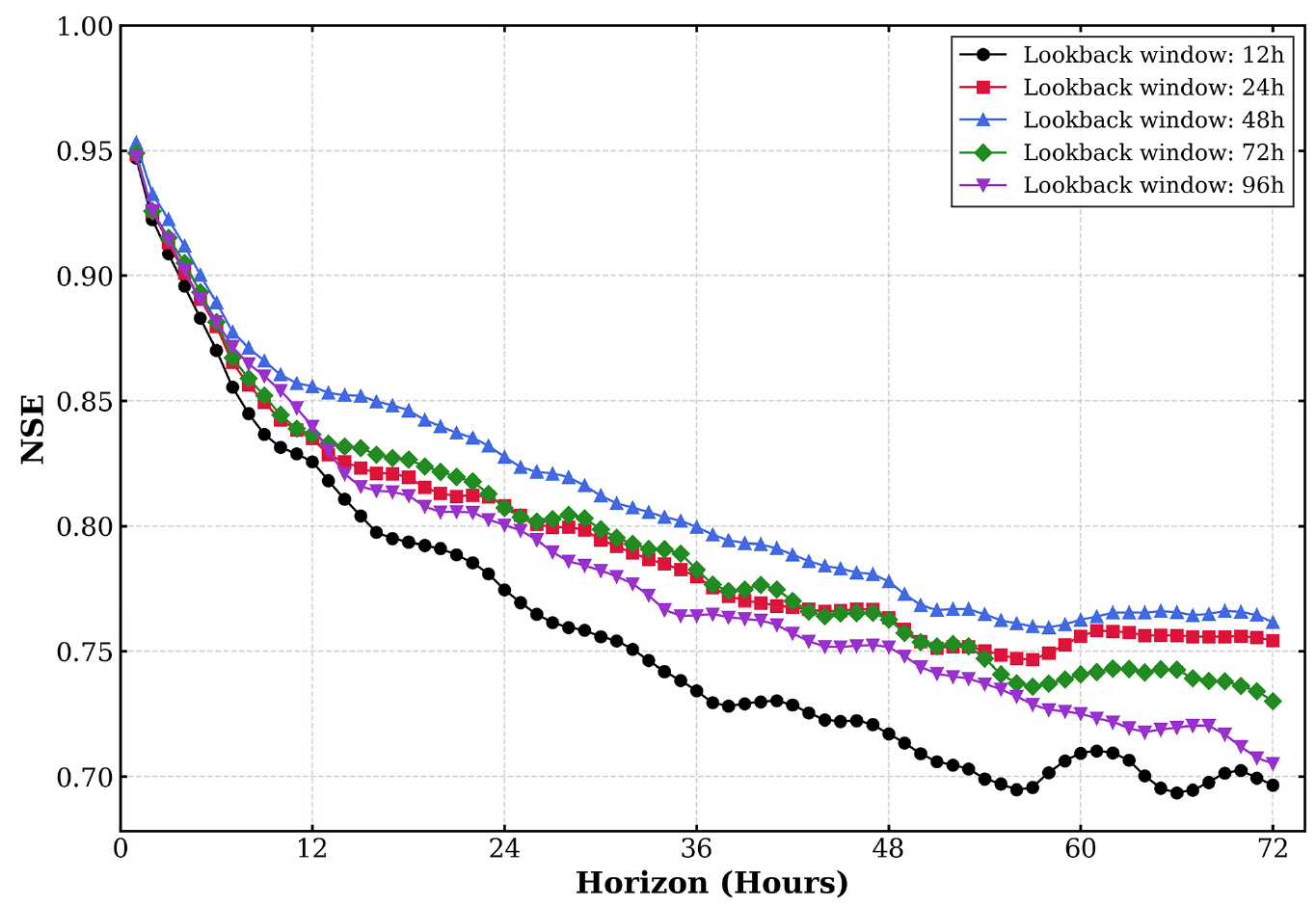
Table 3.
Forecasting performance of the model for the specific forecasting horizons (1, 24, 48, and 72 h) and the overall average (All) under various lookback windows
Among the scenarios, the 48 h lookback window exhibited the best overall performance, achieving the highest average NSE of 0.811 over the entire 72 h forecasting horizon. In addition, it consistently yielded the highest NSE and lowest RMSE at all forecasting time steps, indicating that the 48 h input condition provides an optimal balance between forecasting accuracy and stability (Table 3). In contrast, the 12 h scenario showed a relatively poor performance across all horizons, likely due to its limited ability to capture the lagged and cumulative dynamics of Chl-a variability. Furthermore, the 96 h scenario demonstrated a decline in performance, which could be attributed to the inclusion of excessive historical information, leading to increased noise and computational complexity.
It should be noted that this optimal lookback window is subject to change depending on reservoir-specific characteristics, such as basin area and hydraulic residence time; therefore, it is difficult to generalize this value as a universal biological indicator across different reservoir systems. Rather, the 48 h window in this study represents a site-specific temporal context that enables the model to effectively learn complex non-linear patterns for the Gungpyeong reservoir.
Meanwhile, the scatter plot analysis of the 48 h scenario revealed that the dispersion of the data increased and forecasting uncertainty grew as the forecasting horizon extended. In particular, a vertically concentrated distribution of forecasted values was observed within the range of approximately 20-25 mg/m3, indicating that the model fails to fully reproduce the overall variability of the observed concentrations and tends to converge within a limited range (Fig. 5(b)-(d)). This pattern can be interpreted as a consequence of data imbalance, in which the model becomes biased toward the mean concentration range, resulting in simultaneous underestimation at high concentrations and overestimation at low concentrations (Busari et al., 2023; He and Ma, 2013).
In particular, the limited ability to reproduce high-concentration events is attributed to the exclusion of critical exogenous drivers, such as nutrient concentrations including total nitrogen (TN) and total phosphorus (TP) and inflow/outflow rates. These nutrients are well-recognized as primary limiting factors and triggers for phytoplankton proliferation (Chen et al., 2024; Paerl et al., 2016). However, they were not incorporated in this study due to the lack of continuous monitoring systems in the upstream areas of most agricultural reservoirs. While watershed modeling offers a potential alternative, its reliability remains constrained by the absence of measured data for calibration. Therefore, expanding monitoring networks for these key variables is essential for improving the accuracy of data-driven water quality models. Furthermore, technical strategies such as oversampling techniques to address data imbalance and the adoption of ensemble learning methods should be explored to mitigate the systematic underestimation of peak events (Kim et al., 2025; Zamani et al., 2023).
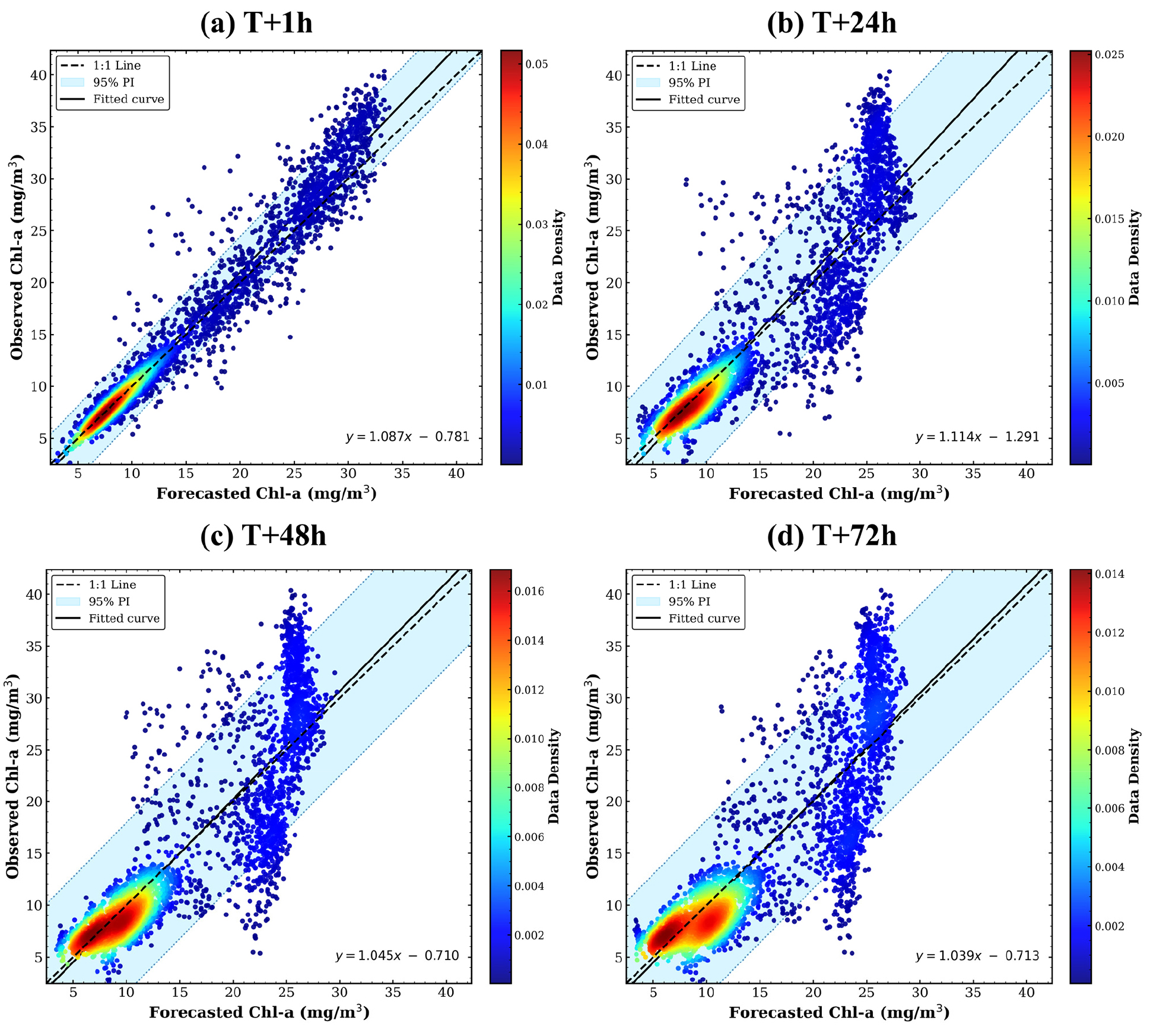
Fig. 5.
Density scatter plots of observed versus forecasted Chl-a across the different forecasting horizons: (a) 1 h, (b) 24 h, (c) 48 h, and (d) 72 h. The dashed black line represents the 1:1 reference, and the solid black line indicates the fitted regression curve. The shaded area bounded by dotted lines denotes the 95% forecasting interval. The color gradient represents the data density based on kernel density estimation.
Interpretation of Forecasting Mechanism based on Cross-Attention
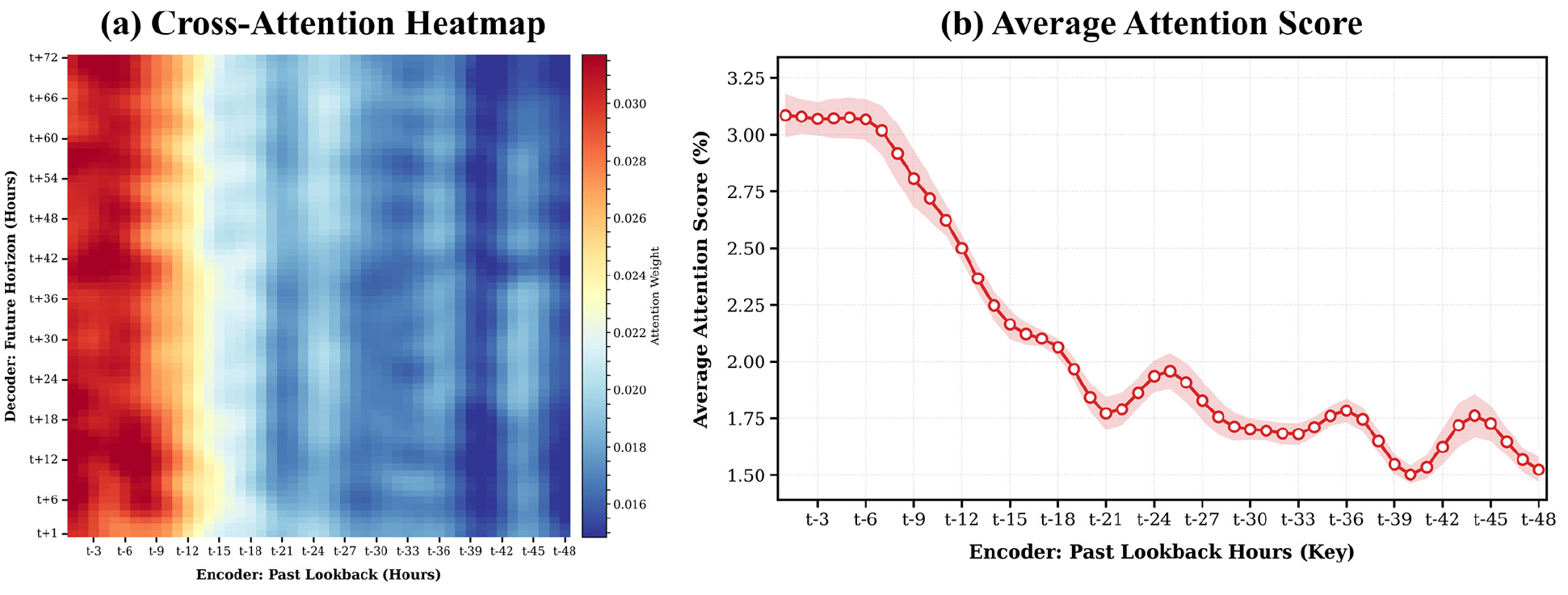
In this study, the cross-attention weight distribution was analyzed to interpret the internal forecasting mechanism of the transformer model developed under a 48 h lookback window condition. The results have shown that regardless of the forecasting horizon (t+1 h-t+72 h), attention weights were consistently concentrated in the most recent past interval (t-1 h-t-7 h), while the weights generally decreased as the temporal distance increased (Fig. 6(a)). This tendency was more clearly confirmed by the average attention score (Fig. 6(b)).
However, the attention weights did not decrease monotonically; instead, localized increases were observed at specific timesteps. In particular, the partial re-emergence of attention weights was identified around t-24 h, t-36 h, and t-44 h, suggesting that the model does not rely solely on recent information but it selectively incorporates temporally relevant past states in a nonlinear manner. This indicates that the model effectively learns a dynamic weighting mechanism that assigns importance to the individual time steps within the input sequence. This behavior highlights the key advantage of Transformer-based models in selectively emphasizing the informative temporal features for forecasting.
Chl-a is known to respond sensitively to meteorological and thermal conditions, even at short (hourly) timescales (Amorim et al., 2021; Blauw et al., 2018), while exhibiting lagged responses and periodic variations. The observed attentional weight distribution was consistent with the temporal dynamics of Chl-a, suggesting that the model appropriately captured its underlying time-dependent characteristics. Therefore, the Transformer architecture is considered effective for modeling highly dynamic water quality time series with complex temporal dependencies.
Conclusion
In this study, a Transformer-based S2S multi-step Chl-a forecasting model for the Gungpyeong reservoir was developed, and the effect of lookback window length on forecasting performance was investigated. The results indicate that increasing the input sequence length does not always improve the performance; excessive historical information can introduce noise and degrade the forecasting accuracy. In particular, the 48 h lookback window was identified as the optimal configuration, providing the best balance between forecasting accuracy and stability. Although the model effectively captured the overall variability patterns, it exhibited a tendency for the forecasted values to converge within a limited range, resulting in an underestimation at high concentrations and an overestimation at low concentrations. This limitation is attributed to data imbalance and insufficient representation of the exogenous factors, particularly external nutrient inflows driven by rainfall, which are critical for reproducing high-concentration events.
From a practical perspective, achieving sufficient forecasting lead times, along with the accurate reproduction of high-concentration peaks, is essential for proactive water quality management. Furthermore, while this study identified a 48 h lookback window as optimal, this duration may vary depending on site-specific characteristics such as watershed scale, reservoir capacity, and regional climatic patterns. Therefore, future research should focus on incorporating exogenous variables, addressing data imbalances, and improving the model architecture to enhance long-term forecasting performance. Additionally, subsequent studies should investigate how these environmental and physical conditions influence the optimal input sequence, thereby ensuring the broader applicability and robustness of the model across diverse reservoir environments. The findings of this study provide a useful basis for designing and applying data-driven water quality forecasting models in reservoir systems.