

Introduction
Materials and Methods
Plant Materials
DNA extraction and genotyping data acquisition
Marker selection methods
Statistical Analysis
Results and Discussion
Summary
Introduction
Doubled haploid (DH) technology enables the rapid development of completely homozygous (2n) lines by generating haploids (n) through artificial crossings with a haploid-inducer line, followed by chromosome doubling (Prasanna et al., 2012). The first widely used inducer, Stock 6, exhibited a 2.9% haploid induction rate. Subsequent advances, including genome editing, led to the development of 24 improved inducer lines, including 19SN952452, which shows an induction rate exceeding 15% (Coe, 1959; Delzer et al., 2024; Ha et al., 2024). In South Korea, tropically adapted inducer lines (TAILs), a subtropical DH inducer have been introduced for maize variety development and applied to develop field, silage, and waxy maize lines (Ryu et al., 2022).
When integrated with genome-wide analysis, DH technology has become a powerful tool for breeding and selection. Large-scale SNP datasets enable detailed assessment of linkage disequilibrium (LD) patterns, haplotype structure, and overall genetic variation. However, several studies have reported reduced genetic variation and loss of variation in DH-derived populations (Strigens et al., 2013; Zeitler et al., 2020). Although using F2 populations can partially alleviate these bottlenecks, offering cumulative selection responses as high as 4%-6% (Bernardo, 2009), this does not necessarily translate into higher heritability or genetic gain (Showkath Babu et al., 2022). Thus, molecular-level evaluation of DH lines is essential within breeding programs. Despite this need, molecular genetic analyses of DH waxy maize lines are limited. This limitation restricts the development of core SNP marker sets critical for efficient variety management and genetic diversity assessment. Given the large volume of SNPs generated in modern genomic workflows, selecting a small, representative set of core SNP markers is essential for practical use in breeding, germplasm characterization, and resource management (Du et al., 2019; Fujii et al., 2013; Li et al., 2019; Varshney et al., 2008). Existing DH-based studies often examine isolated genetic metrics, such as LD decay, genetic distance, or population structure, without providing comprehensive whole-genome evaluations of genetic diversity, LD structure, and core marker selection strategies using large-scale SNP datasets. Furthermore, most previous studies have relied on field corn or experimental DH populations, limiting the relevance of findings to domestically bred Korean waxy maize DH resources.
Therefore, in this study, we aimed to overcome these limitations by characterizing LD extension and diversity reduction in DH-derived waxy maize lines. Furthermore, we sought to identify a practical, representative core SNP marker set from genome-wide SNP data. To achieve this, we quantified population genetic characteristics of DH lines, compared three marker selection algorithms, and evaluated their applicability in breeding programs.
Materials and Methods
Plant Materials
A total of 155 waxy maize lines were used in this study, including 26 elite lines used for variety development (Ilyas et al., 2023; Park et al., 2009; Sa et al., 2010), 18 inbred lines derived from selfed full-sib heterotic group populations (Park et al., 2016), and 111 lines developed through DH technology (Table 1). To induce DH lines, the hybrid Mibaek 2 (Park et al., 2007) and Gangwonchal 39 were used in 2016. In 2017, segregating generations derived from the half-sib heterotic group served as breeding material. In 2018, hybrid combinations classified as resistant or susceptible based on inoculation with Fusarium subglutinans and F. temperatum, the causal agents of corn stalk rot, were used to generate additional DH lines.
Table 1
Summary of the 155 waxy maize lines used for SNP selection
DNA extraction and genotyping data acquisition
Young leaf tissue collected from pot-grown plants was freeze-dried (IlShinBioBase, South Korea), homogenized using a Tissue Lyser II (Qiagen, Germany), and used for genomic DNA extraction using the QIA Symphony SP platform with the QIA Symphony DSP DNA Mini Kit (Qiagen) according to the manufacturer’s instructions. Genotyping was performed using the Illumina MaizeSNP50K BeadChip (Illumina, USA). After manufacturer-recommended filtering and removal of SNPs not mapped to waxy maize chromosomes, 49,037 SNPs were obtained. Further filtering excluded markers with ≥ 10% missing data, monomorphic loci, and SNPs with ≥ 20% heterozygosity, resulting in a final dataset of 21,981 SNPs for downstream analysis.
Marker selection methods
To select core SNP markers suitable for waxy maize, three previously reported marker selection strategies were applied and compared. First, the index-based method was implemented using the Shannon entropy formula (Dou et al., 2023).
In this formula, n denotes the number of alleles or genotypes, and pi represents the frequency of the i-th allele or genotype. Haplotypes were iteratively constructed from candidate SNPs, and the stepwise increase in the Shannon index (SI) was used to evaluate each newly added marker. At each iteration step, we added one remaining candidate marker to generate a new haplotype set and calculated the resulting increase in the Shannon index. The marker producing the greatest increase in SI was selected as the next core marker. If adding a candidate marker did not increase the number of distinguishable haplotypes, that SNP was excluded to improve algorithmic efficiency. The procedure terminated when all line pairs were distinguished or when no further increase in the index was observed. The second method, described by Wu et al. (2021), used random sampling of SNPs to calculate Euclidean genetic distances across all lines and identify subsets that maximized the minimum pairwise genetic distance (random sampling with genetic distance, RS). The number of markers (K) ranged from 10 to 100. For each k, 6.0 × 10⁵ subsets were sampled, increasing to 1.0 × 10⁷ times for k ≥ 20. If classification power did not improve after a predefined number of iterations, the algorithm moved to the next value of k. When no additional improvement was observed across increasing k, the subset with the best performance was selected. The third method employed a fitness function incorporating genetic distance (gd) and physical distance (pd) to ensure a uniform chromosomal distribution of markers (Rousselle et al., 2015). Genetic map positions from the IBM and LHRF populations in MaizeGDB were used, and only SNPs with both physical and genetic coordinates were retained. To avoid bias introduced by specific cross combinations, polymorphisms present only in HW3 and HW9 were excluded. The optimization process was iterated to identify the marker panel that consistently minimized the fitness value.
Statistical Analysis
Allele frequencies were estimated for each SNP after excluding missing data using q = 1 - p. Minor allele frequency (MAF) was defined as MAF = min(p,q), polymorphism information content as (PIC) = 2pq(1 - pq), and expected heterozygosity as He = 2pq. We calculated the mean number of alleles per group and identified group-specific alleles that were found only within each group. Population differentiation (Fst) was estimated using the Weir and Cockerham (1984) method implemented using the R package hierfstat (R Core Team, 2023). For phylogenetic tree analysis, a genotype matrix was constructed for each marker set. Inter-line genetic identity (I) was calculated and transformed to -ln(I) to obtain Nei’s genetic distance (Nei, 1972). Neighbor-Joining (NJ) trees were constructed from the resulting distance matrix using the ape package in R. To validate NJ results, we calculated the nearest-neighbor purity (NN-purity), defined as the proportion of tips whose nearest neighbor belonged to the same group (Degen et al., 2017). A null distribution was generated from 1,000 random permutations of group labels, from which the mean, standard deviation, and Monte Carlo p-value were estimated. For principal coordinate analysis (PCoA), Nei’s genetic distance matrix was was analyzed by eigenvalue decomposition using the ape package. The variance explained by positive eigenvalues was calculated, and the first two coordinates (PCoA1 and PCoA2) were used for visualization. When negative eigenvalues were significant, Cailliez/Lingoes correction was applied.
LD was calculated for all SNP pairs within each chromosome up to 5 Mb. To reduce computational load for visualization, distance-based bin subsampling was applied (10 kb bins, up to 300 pairs per bin). The SNP matrix was processed in blocks of 512 SNPs, and pairwise r2 values were calculated as the squared Pearson correlation coefficient, using only SNP pairs with at least 12 valid samples. Haplotype frequencies were estimated using the expectation-maximization (EM) algorithm, and statistical significance was assessed with Fisher’s exact test followed by Benjamini–Hochberg correction. LD decay was visualized by plotting median r2 values within 50-kb physical distance bins. Mean LD distance (r2 ≥ 0.10) was summarized in heatmaps across groups and chromosomes. SNP-specific MAF values were matched to LD values to compare LD decay under increasing MAF thresholds (≥ 0.00, 0.05, 0.10, and 0.20) in the 18DHW group. Group-wide LD distributions were visualized using violin plots to compare median and variance. All numerical statistics (median r2 and mean LD distance) were derived from full-matrix calculations, whereas the figures present subsampled summaries for visualization (Benjamini and Hochberg, 1995; Pe’er et al., 2006; Remington et al., 2001; Stephens et al., 2001; VanLiere and Rosenberg, 2008). All data analyses were conducted using R.
Results and Discussion
The SNP markers used in this study ranged from 1,485 to 3,485 per chromosome after filtering. Chromosome 1 contained the highest number of markers (3,485), whereas chromosome 10 contained the lowest (1,485). The physical distance between adjacent markers ranged from 86 to 100 kb, with an average of 94 kb. Mean heterozygosity across chromosomes was 1.4%, with chromosome 4 showing the highest value (2.0%) and chromosome 6 the lowest (1.0%) (Table 2).
Table 2
Chromosome-wide SNP filtering and genomic statistics in waxy maize lines
| Chromosome |
Number of raw SNPs |
Number of filtered SNPs |
Mean distance of filtered SNPs (bp) |
Heterozygosity rate (%) |
| 1 | 7,783 | 3,485 | 86,397 | 1.3 |
| 2 | 5,667 | 2,497 | 95,216 | 1.6 |
| 3 | 5,525 | 2,509 | 92,387 | 1.2 |
| 4 | 5,411 | 2,428 | 99,612 | 2.0 |
| 5 | 5,349 | 2,500 | 87,096 | 1.1 |
| 6 | 3,935 | 1,757 | 96,272 | 1.0 |
| 7 | 4,062 | 1,890 | 93,183 | 1.4 |
| 8 | 4,231 | 1,864 | 94,053 | 1.6 |
| 9 | 3,598 | 1,566 | 99,923 | 1.4 |
| 10 | 3,476 | 1,485 | 100,391 | 1.2 |
| Overall1) | 49,037 | 21,981 | 94,453 | 1.4 |
Among genetic diversity metrics, elite lines showed the highest number of group-specific alleles (1,432) and the greatest expected heterozygosity (He = 0.315) (Table 3). High He values were also present in the heterotic full-sib group (0.268) and the 17DHW group (0.273). In contrast, the 18DHW population, derived from crosses between stalk rot-resistant and susceptible lines, exhibited the lowest values across all diversity metrics except for the count of specific alleles.
Table 3
Genetic diversity metrics across groups. Values represent locus-wise means for MAF, PIC, He, and the number of group-specific alleles
| Group | MAF | PIC | He | Specific alleles |
| Elite line | 0.234 | 0.254 | 0.315 | 1,432 |
| Inbred | 0.202 | 0.214 | 0.268 | 51 |
| 16DHW | 0.160 | 0.174 | 0.216 | 97 |
| 17DHW | 0.204 | 0.219 | 0.273 | 91 |
| 18DHW | 0.152 | 0.141 | 0.182 | 112 |
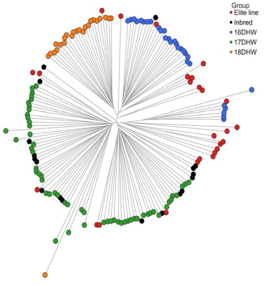
Phylogenetic analysis based on Nei’s genetic distance revealed that most lines formed well-defined, continuous clusters (Fig. 1). Elite lines were broadly separated into two groups, whereas the inbred lines were more widely dispersed and generally positioned between the DH groups. Some elite and inbred lines clustered very closely on the tree and were presumed to have originated from a common source during line development. The nearest-neighbor purity (NN-purity) was 86.5%, significantly higher than the permutation-based 23.5% ± 3.9% (p < 0.001). This strongly supports the presence of a well-defined and robust group structure.
The elite lines and inbred groups showed rapid LD decay, whereas the 18DHW group maintained r2 values around 0.5 even at distances up to 5 Mb, exhibiting a pronounced long-range LD pattern (Fig. 2a). To examine whether allele-frequency differences contributed to this extended LD in the 18DHW population, we evaluated LD estimates under increasing MAF thresholds (Fig. 2b). Group-wide LD distributions were also summarized to compare LD patterns among groups (Fig. 2c). To confirm these patterns were not artifacts of IBD or LD dependence, identity-by-descent (IBD) was estimated using an EM-based maximum likelihood method with an LD-pruned SNP set (r2 ≤ 0.20). The maximum estimated IBD value (π) reached 0.997. PCA coordinates before and after LD pruning showed strong concordance (Procrustes t0 = 0.971), indicating that the inferred population structure is highly robust despite elevated pairwise IBD and LD-related dependence. Even when the MAF threshold was increased in the 18DHW group, the overall LD decay curve remained largely unchanged. The violin plot revealed consistently high r2 values across the distribution, indicating that many SNP pairs exhibit strong LD. These results suggest that the long-distance LD observed in this population cannot be attributed solely to statistical fluctuations arising from rare variants but is instead consistent with underlying genetic features of the group (Flint-Garcia et al., 2003; Remington et al., 2001). More detailed analyses, such as removing identical sequences, accounting more explicitly modeling relatedness using IBD estimates, or clumping physically adjacent SNPs, may be necessary for deeper investigation of this extended LD architecture.
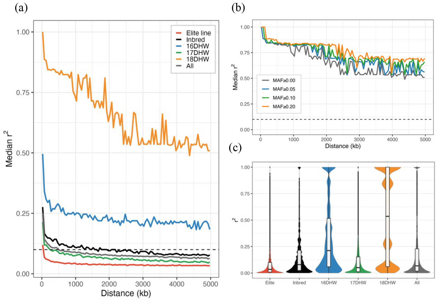
Fig. 2.
Linkage disequilibrium (LD) patterns across groups. (a) LD decay curves showing the median pairwise r2 within 50 kb physical distance bins for each group; the horizontal dashed line indicates r2 = 0.10 as a reference threshold. (b) LD decay in the 18DHW group stratified by minor allele frequency (MAF) thresholds (MAF ≥ 0.00, 0.05, 0.10, 0.20), illustrating the expected increase in r2 under stricter MAF cutoffs. (c) Violin plots depicting the distribution of pairwise r2 values in each group; embedded boxplots indicate the median (central line) and interquartile range (box).
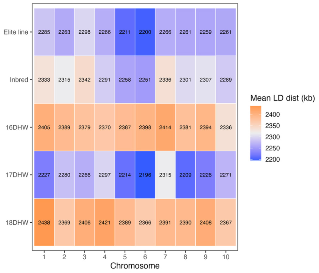
Analysis of the mean LD distance per chromosome revealed that the elite and inbred groups exhibited short LD distances ranging from 2,200 to 2,298 kb. However, the 18DHW group showed the largest mean LD distance, reaching 2,438 kb on chromosome 1 (Fig. 3). Hao et al. (2015) reported LD lengths of 1,500-2,000 kb in a Chinese waxy maize population, which is comparable to the results observed in our study. Previous studies have also shown LD expansion in haploid populations derived from wild-type maize, where genetic diversity was markedly reduced due to allele loss at both nucleotide and haplotype levels (Zeitler et al., 2020). These findings are consistent with our results and suggest that the use of DH technology may contribute to LD expansion, underscoring a need for improvement in breeding programs that rely heavily on DH lines. Although the 18DHW group maintained clear long-distance LD in the decay curve, the mean LD distance measured only approximately 2,395 kb. This discrepancy reflects differences in the statistical properties of LD metrics and mirrors patterns reported in plant-population studies (Brazier and Glémin, 2022). Although the mean LD distance is relatively low due to the abundance of short-range LD pairs (Remington et al., 2001), strong LD was still maintained across certain long-distance genomic regions (Epstein et al., 2024; Palaisa et al., 2004). This phenomenon can be explained by reduced effective population size, inbreeding, or selection acting on genomic segments with low recombination rates (Bukowski et al., 2018). Therefore, selecting an optimized marker set requires strategies that reduce SNP redundancy caused by long-range LD while preserving marker information content (Carlson et al., 2004; Takeuchi et al., 2005) and minimizing the total number of markers required (Paschou et al., 2010; Rosenberg et al., 2003).
To characterize differences among groups, we assessed population differentiation and genetic distance using Nei’s distance (Table 4). 18DHW and 16DHW showed the greatest genetic distance (Nei’s distance = 0.285), whereas the 17DHW-inbred group showed the lowest Fst and genetic distance (both 0.009), reflecting the shared breeding line used in their development. Although the 18DHW group exhibited low within-group genetic diversity (Table 3), the high between-group genetic distances and Fst values suggest that genetic differentiation may have increased in response to selection for disease resistance. This pattern aligns with previous reports showing that repeated selection within a group decreases internal diversity while increasing differentiation from other groups (Ledesma et al., 2023). The elite group exhibited the highest within-group genetic diversity (Table 3) but showed intermediate levels of differentiation from other groups. This pattern is reminiscent of U.S. commercial maize breeding, where a limited set of founder lines was repeatedly used to develop improved varieties. As a result, founder haplotypes occur at high frequency across derived germplasm (Coffman et al., 2020; Van Heerwaarden et al., 2012). Collectively, these findings indicate that increasing genetic diversity should be a priority in breeding programs. For DH populations under strong selection pressure, incorporating external founder lines or different LD blocks will be essential to maintain diversity and ensure long-term breeding progress.
Table 4
Pairwise genetic differentiation (Fst) and genetic distance among elite lines, inbreds, and DH groups
This intergroup differentiation pattern suggests that core marker selection should prioritize group discrimination and genome-wide coverage over simple diversity metrics. Based on these molecular analyses, we applied three marker-selection methods—the Shannon index (SI), random sampling with genetic distance (RS), and map-based balanced (bin) approaches—to derive highly informative SNP panels.
Ten markers were selected through the SI-based screening, enabling clear discrimination of haplotypes across 155 lines (Fig. 4a). The RS method achieved a maximum classification ability of 99.98% (Fig. 4b). This limitation occurred because three line pairs (18DHW025-18DHW026, 16DHW01-16DHW04, and 16DHW25-16DHW29) were identical across all non-missing loci, and another pair (16DHW25–16DHW29) differed at only one SNP.
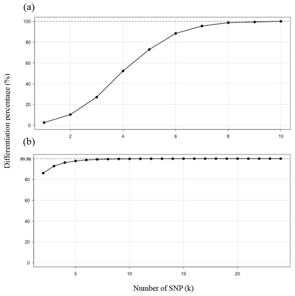
Fig. 4.
Discrimination saturation curves as a function of the number of SNPs (k). The y-axis shows the proportion of pairwise sample comparisons that are distinguishable. (a) Shannon index (SI) selection evaluated by haplotype separation. (b) Random sampling with genetic distance (RS) selection evaluated using Euclidean genetic distance. The dashed line indicates the maximum discrimination achieved for each curve (SI: 100.0%; RS: 99.98%).
We visualized the physical distribution of markers selected across all 10 chromosomes for the SI, RS, and bin-based methods (Fig. 5). The small number of SNPs selected by SI and RS methods resulted in coverage of only a subset of chromosomes, whereas the bin-based selection produced broad chromosomal coverage as the number of markers increased. These results demonstrate that the bin-based method has a particular advantage for achieving whole-genome representativeness, while also highlighting that each selection method carries distinct strengths and weaknesses in classification performance. Notably, we observed overlapping marker selection from all three methods on chromosome 1. This biased distribution suggests chromosome-specific structural features, such as recombination rate variation, gene density, or repetitive elements. Further investigation of these genomic characteristics could help explain the uneven distribution and clustering of selected markers. Overall, our results suggest that core SNP marker selection should balance strong classification performance with uniform genomic coverage to construct an informative and representative marker panel.
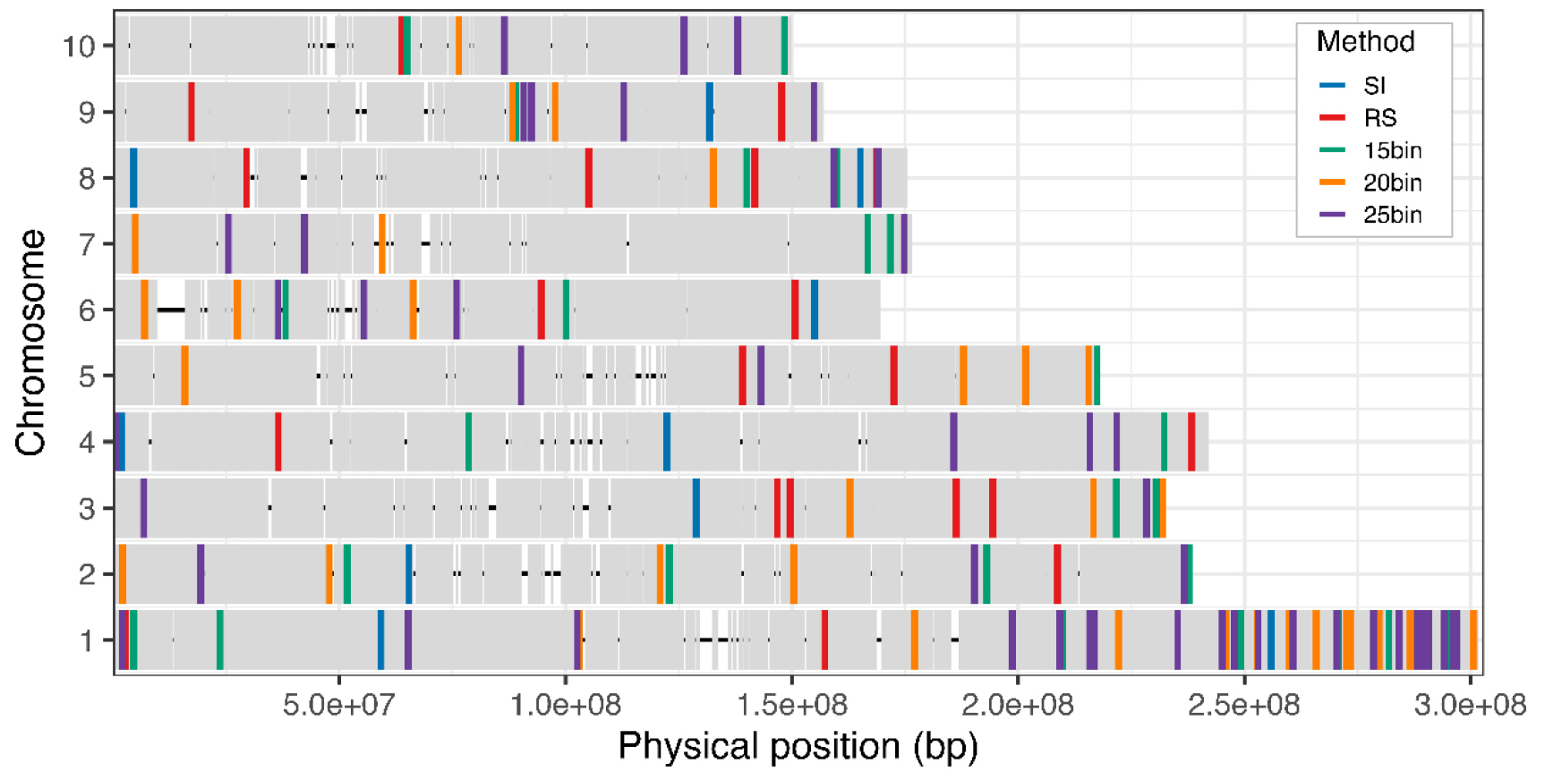
Fig. 5.
Chromosomal distribution of SNPs selected using each marker selection method: SI (n = 10), RS (n = 21), 15bin (n = 30), 20bin (n = 39), and 25bin (n = 47). Gray ticks indicate the filtered whole-genome SNP background; colored bars correspond to the SNPs selected using each method as shown in the legend.
To evaluate the selection efficiency of the marker panels, we calculated standard genetic diversity metrics (Table 5). The SI-based approach generated the smallest panel (10 markers) but achieved the highest performance across all metrics—MAF, PIC, and expected heterozygosity—because it prioritizes high-MAF markers through entropy-based selection. The 21-marker RS panel showed intermediate levels across all three diversity metrics. In contrast, the bin-based panels, which select markers solely based on genetic and physical distance, displayed lower diversity relative to the full filtered SNP set. The 20bin panel (39 markers) had the lowest values across all metrics, suggesting that distance-based selection inadvertently included SNPs with overlapping LD or rare alleles.
Table 5
Summary statistics for SNP marker sets obtained using each selection strategy. Values represent the number of selected markers and mean diversity indices (MAF, PIC, and expected heterozygosity (He)).
| Method1) | Number of markers | MAF | PIC | He |
| Filtered | 21,981 | 0.221 | 0.240 | 0.299 |
| SI | 10 | 0.374 | 0.329 | 0.434 |
| RS | 21 | 0.254 | 0.275 | 0.343 |
| 15,000 | 30 | 0.176 | 0.209 | 0.253 |
| 20,000 | 39 | 0.148 | 0.187 | 0.223 |
| 25bin | 47 | 0.208 | 0.245 | 0.299 |
1)Methods: SI: Shannon index-based selection; RS: random sampling with genetic distance maximization; 15bin/20bin/25bin: genome-wide binning by genetic/physical coordinates targeting 15, 20, or 25 bins. Abbreviations: MAF: minor allele frequency; PIC: polymorphism information content; He: expected heterozygosity.
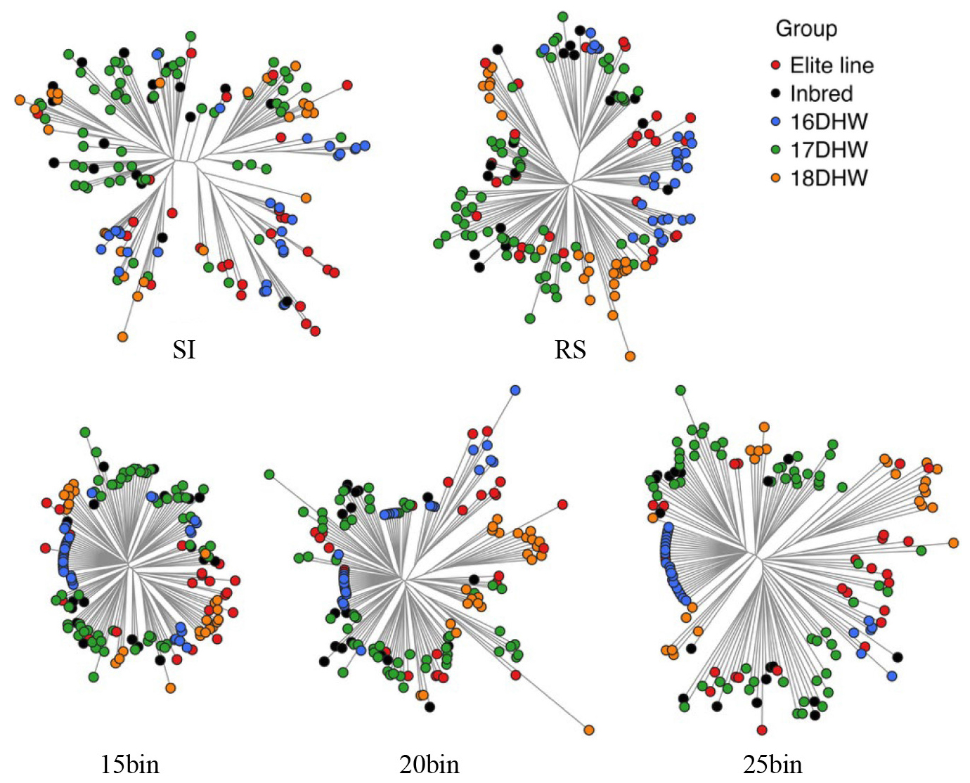
We examined phylogenetic separation using NJ trees constructed from Nei’s genetic distance (Fig. 6). The SI panel provided good individual-level resolution but showed limited discrimination among groups, with frequent intermixing of elite and DH lines. Bin-based marker sets also enabled clear group-level differentiation. DH lines formed distinct clusters under both the RS and bin marker panels, reflecting their differing genetic backgrounds. In contrast, elite lines were distributed across diverse positions within the inbred and DH clusters, indicating their broad use across breeding programs and substantial genomic contribution, likely due to shared founders or repeated use in line development. These results indicate that a marker panel of appropriate size can effectively capture population structure and classify lines within breeding programs.
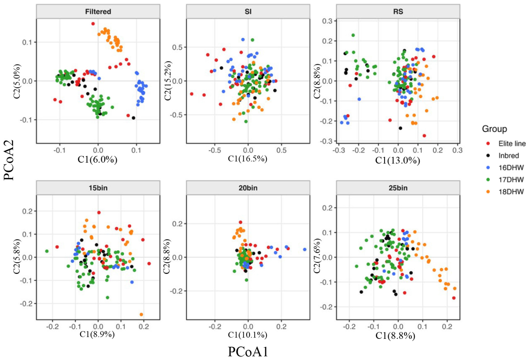
Additionally, we evaluated the population structure of the 155 lines using PCoA based on each selected SNP panel (Fig. 7). Analysis using the filtered whole-genome markers revealed clear separation among groups and among lines within groups, indicating effective capture of intergroup genetic variation. In contrast, the SI-based panel did not achieve clear separation of breeding groups. Although SI markers were highly polymorphic, they did not maximize between-group contrast, resulting in weaker cluster differentiation. The RS panel, despite being composed of randomly sampled markers, achieved better group separation than SI because it captured intergroup variation. Among the bin-based panels, the 25bin panel produced more distinct clustering and clearer group separation than the 20bin panel, while the 15bin panel exhibited only limited group-level resolution. The 20bin panel showed the lowest classification ability, with most samples clustering near the origin. These results indicate that increasing the number of markers does not guarantee improved PCoA resolution in bin-based methods. In contrast, the 25bin panel provided improved separation power within the bin-based framework. Because DH lines exhibit low expected heterozygosity and long-range LD, many SNPs provide redundant information. Therefore, selecting uncorrelated markers distributed across the genome is essential for accurately capturing relative genetic distances among lines using a small marker set. Furthermore, SNPs selected solely based on diversity do not always provide strong discriminative power (Nei, 1972; Rosenberg et al., 2003; Sodedji et al., 2021). Previous studies have shown that a small number of highly informative SNPs, identified through measures such as PCA loadings or Fst, can effectively replicate the population structure captured by large genome-wide SNP datasets (Flint-Garcia et al., 2003). Future marker selection strategies should incorporate these considerations.
Summary
The application of DH technology in waxy maize breeding enables rapid development of fully homozygous lines but also reduces genetic diversity and increases LD extent. To improve the efficiency of DH-based breeding programs, we evaluated molecular characteristics across groups with different breeding histories and assessed phylogenetic structure and genetic diversity. Core marker selection was performed using three complementary algorithms. Although SI markers were highly diverse, they provided insufficient group-level discrimination, limiting their classification utility. RS markers showed superior discriminatory power by optimizing genetic distance. Although the bin-based method offered lower classification power, it provided balanced genome-wide representation. Overall, the 21-marker RS panel effectively captured both line-level classification and population structure. When combined with markers that enhance chromosomal coverage and diversity, this panel can improve the accuracy and efficiency of routine genotyping in breeding programs. We plan to further evaluate the classification performance of the selected markers using large-scale genotyping platforms including applications to DH lines and lines derived from segregating generations. This core SNP panel provides a ready-to-use tool for quality control and resource management, such as line identification, variety protection, core population management, and seed purity testing. Ultimately, these tools will support the establishment of a core waxy maize germplasm set and contribute to the development of a next-generation waxy maize breeding platform.
