Introduction

Perilla (Perilla frutescens L.) is an oilseed and vegetable crop primarily cultivated in Korea, China, India, and East Asia. The seeds of perilla contain a high oil content (35－45%) and are rich in alpha-linolenic acid, making them an important functional plant resource for human health (Shin and Kim, 1994; Yu et al., 2017). The leaves of perilla are rich in polyphenols such as anthocyanins and rosmarinic acid and exhibit strong antioxidant activity (Fujiwara et al., 2018; Lee and Shin, 2024).

However, domestic perilla cultivation faces substantial threats to productivity due to blight caused by Phytophthora infection, as well as water stress resulting from drought and waterlogging, both of which are exacerbated by climate change. Phytophthora is an oomycete that produces zoospores; it spreads rapidly under warm, humid conditions and infects plants by entering through the roots and stem base or via leaf stomata during rainfall (Lamour et al., 2012; Wu et al., 2020). Because Phytophthora blight causes symptoms associated with water supply disorders—such as wilting, yellowing, and leaf scorch—its visual manifestations closely resemble those of water stress caused by drought or over-irrigation. Consequently, distinguishing between blight and water stress remains challenging through visual inspection alone (Hornero et al., 2021; Pscheidt, 2023). These diagnostic challenges lead to the misuse of pesticides and improper cultivation practices; thus, accurate classification techniques are necessary.

Hyperspectral imaging (HSI) is a non-destructive technique that captures continuous spectral information from the visible to the near-infrared spectrum on a pixel-by-pixel basis, enabling the detection of changes in chlorophyll content, cellular structure, and moisture content before visible symptoms appear (Lowe et al., 2017). Recently, for the early diagnosis of leaf blight in sesame, a 3 × 3 patch-based spatio-spectral integrated analysis method was applied using visible and near-infrared (400－1,000 nm) hyperspectral imagery. Please move the reference for (Kang et al., 2025) to the appropriate location. In the field of environmental stress, drought stress tolerance was evaluated in cotton varieties using hyperspectral imagery and a one-dimensional convolutional neural network (1D-CNN). Key spectral indicators included the green reflectance peak was in the visible waveband (520－580 nm) and alterations in cellular structure reflected in the near-infrared region (760－1,250 nm). Among ten evaluated algorithms, the 1D-CNN demonstrated superior predictive performance (Guo et al., 2022; Kang et al., 2025).

A paucity of research exists regarding hyperspectral imaging-based methods that simultaneously diagnose blight and water stress in perilla plants. Therefore, this study aimed to develop a technique for the non-destructive classification of perilla blight, water deficiency, and waterlogging using hyperspectral imagery, Partial Least Squares Discriminant Analysis (PLS-DA), and 1D-CNN. In particular, we analyzed and classified the spectral characteristics of four treatment groups, including diseases that cause similar above-ground symptoms and water stress, using unsupervised and supervised learning. Additionally, we compared and analyzed changes in classification performance across different stages of stress progression, from early stages with no apparent visual manifestations, to later stages exhibiting distinct symptoms.

Materials and Methods

Plant Materials and Experimental Design

The “Anyu” cultivar of P. frutescens L. was used as the reference material for the experiment; it was obtained from the National Institute of Food Science and Technology at the Rural Development Administration. The seeds were disinfected for 2 min in 70% ethanol, followed by 2 min in a 0.1% sodium hypochlorite solution, then rinsed thrice with sterile water. After sowing, the seeds were grown for 4 weeks, and the seedlings that reached the three-leaf stage were selected and transplanted into plastic containers (248 mm width × 180 mm length × 93 mm height) filled with general-purpose horticultural potting mix, and then grown in a growth chamber. The cultivation conditions were 28/25°C (day/night), with a relative humidity of 30－80%, a photoperiod of 16/8 h (light/dark), and a light intensity of 12,000－15,000 lux. Twenty-five plants were used per treatment.

Stress Management

The control group received irrigation once a day. In the drought treatment group, irrigation was discontinued starting on day 0 to induce soil water deficiency. For the waterlogging treatment, a plastic container was placed inside an external container filled with water; perforations were drilled into the base of the internal container to maintain waterlogged soil conditions through a continuous inflow of water. The water level in the outer container was maintained at the same level as the soil surface. The Phytophthora nicotianae MR40622 strain was initially cultured on V8 agar at 25°C for 7 days, after which a culture fragment (1 cm × 1 cm) was inoculated into 700 mL of V8 liquid medium and subjected to secondary culture at 25°C, 130 rpm for 10 days. The culture medium was inoculated into the perilla soil using the soil drenching method as established by Afroz et al. (2019). Hyperspectral images were captured at the same time each day starting from the first day of treatment. Images were captured from days 0 to 10 for the control, drought, and waterlogging treatment groups, and from days 0 to 5 for the Phytophthora treatment group, due to the fast progression of disease.

To build the classification model, the data were categorized by the number of days elapsed after processing. The control, drought, and waterlogging treatment groups were classified into early (days 0－3), middle (days 4－7), and late (days 8－10) stages based on visibility of symptoms, while the Phytophthora treatment group was classified into early (days 0－2) and late (days 3－5) stages. Since the Phytophthora treatment group was divided only into two stages, the late-stage data were applied separately when constructing principal component analysis (PCA) and classification models for the mid- and late-stage data.

Hyperspectral Image Acquisition

Hyperspectral images were acquired using a SPECIM FX10e sensor (SPECIM Ltd., Finland). Spectral information was provided across 224 contiguous bands in the 400－1,000 nm range using a line-scan method with 1,232 spatial pixels. For the imaging system, a plastic container was placed above the sample stage under darkroom conditions, and the conveyor belt speed was adjusted to ensure optimal spatial resolution based on working distance. Two halogen lamps were positioned at a 45° angle to minimize specular reflection (Fig. 1). The measurements were taken at the same time each day to minimize variations due to plant circadian rhythms. Five specimens were placed in a single frame and photographed simultaneously. A white reference image using a 99% standard white plate (Spectralon, Labsphere Inc., USA) and a dark-current image were acquired before each scan for spectral calibration. The reflectance was calculated using Eq. (1):

where R denotes the corrected reflectance image, I_o denotes the original image, I_d denotes the dark current image, and I_w denotes the white reference image.

Fig. 1.

Hyperspectral imaging system.

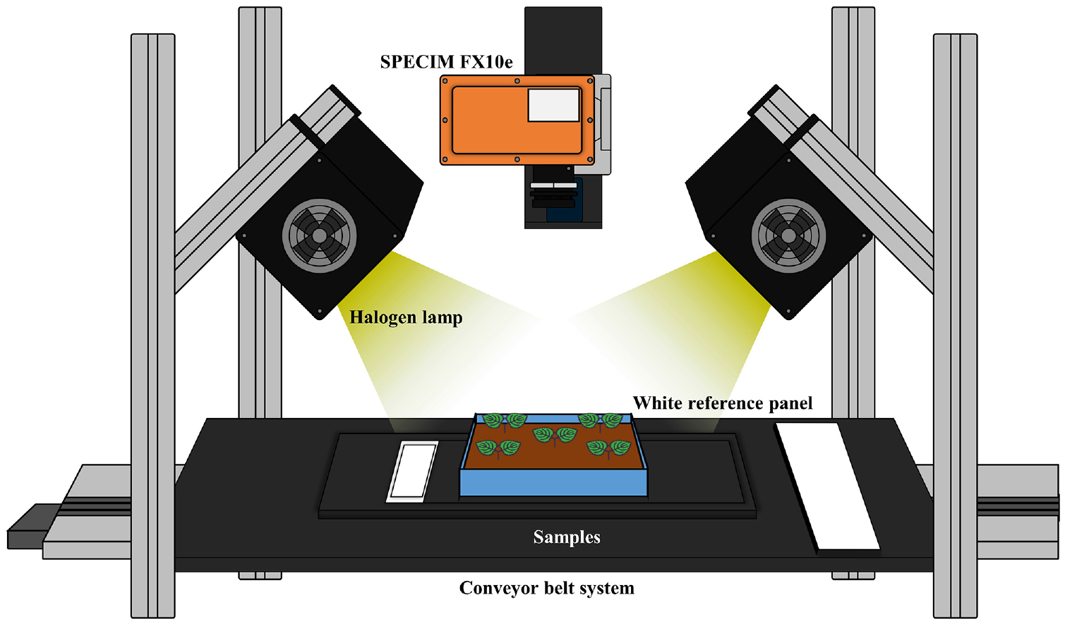
Hyperspectral Image Processing

To determine leaf area from hyperspectral images, the reflectance ratio between the 670 nm and 800 nm wavelength bands was calculated, and the Otsu threshold was applied to segment the vegetation from the background. A connection-based analysis was performed on the extracted leaf regions to isolate individual objects, and small regions measuring less than 50 pixels were removed. For every pixel in each image, a treatment label was assigned based on the experimental design; these pixels were used as the training data for the corresponding treatment. Of the 224 bands in the 400－1,000 nm range, only 184 bands in the 450－950 nm range were used in the analysis, to eliminate noise. Hyperspectral image processing yielded approximately 16 million pixels from 25 individuals per treatment group.

Spectral Preprocessing

To ascertain an optimal preprocessing method, four preprocessing methods were implemented on the extracted spectral data: raw reflectance, Savitzky－Golay smoothing (SG; window length = 11, polynomial order = 2), Standard Normal Variate (SNV), and 1st derivative (window length = 11, polynomial order = 2).

PCA

PCA was performed to exploratively examine differences in spectral patterns among treatment groups based on pretreatment methods and stage of stress progression. PCA is an unsupervised learning technique and was performed without label information for the treatment groups. Following calculation of the mean spectra for each distinct region of the objects that were separated during hyperspectral image processing, normalization was applied, and the top two principal components (PC1 and PC2) were extracted, which were then visualized as a score plot. In the visualization, the treatment group information was assigned to each data point to examine cluster distribution.

Building the Classification Model

The preprocessed spectral data were stratified at the object level and divided into training, validation, and test sets in a 6:2:2 ratio. The validation set was used to select the optimal number of latent variables for PLS-DA and to determine the early stopping threshold and learning rate for the 1D-CNN, while the final classification performance was evaluated using the test data set. Data leakage between objects was prevented by ensuring that all pixels of the same object were placed in the same set. The model was trained at the pixel level.

PLS-DA is a supervised dimension reduction technique that performs classification by extracting latent variables that maximize the variance between classes in high-dimensional spectral data (Barker and Rayens, 2003). The optimal number of latent variables was automatically selected as the value that yielded the highest accuracy on the validation set within the range of 2－20.

1D-CNN is a deep learning technique that learns local patterns in one-dimensional time-series or spectral data, and which effectively extracts correlations between wavelengths in spectral data (Kiranyaz et al., 2021). The model was implemented using the PyTorch framework and consisted of three convolutional blocks, a Global Average Pooling layer, and two fully connected layers (Fig. 2). Each convolution block consisted of a 1D convolutional layer, batch normalization, ReLU, and dropout. The training parameters were set to a batch size of 128, a maximum of 300 epochs, a learning rate of 0.001, and a weight decay of 1 × 10^-5, and the ReduceLROnPlateau scheduler and early stopping (patience = 30) were applied.

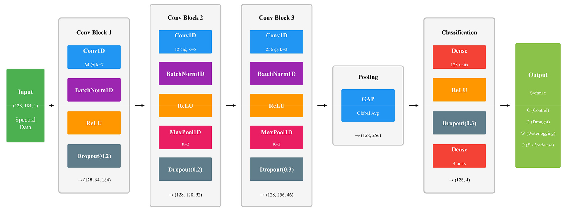
Fig. 2.

Architecture of the one-dimensional convolutional neural network (1D-CNN) model used for pixel-level spectral classification. The model consisted of three convolutional blocks (with 64, 128, and 256 filters), Global Average Pooling (GAP), and two fully connected layers for four-class classification. BN: Batch Normalization, ReLU: Rectified Linear Unit, FC: Fully Connected Layer.

Model Evaluation

Performance of the classification model was evaluated using the test data set, with accuracy and F1-score serving as the primary evaluation metrics. The F1-score was calculated as the harmonic mean of precision and recall as per Eqs. (1), (2), (3), (4), (5):

where TP, TN, FP, and FN denote true positive, true negative, false positive, and false negative, respectively.

Results and Discussion

Spectral Reflectance Characteristics by Treatment Group

Hyperspectral image data were acquired for the four treatment groups—control, drought, waterlogging, and Phytophthora—and the spectral reflectance characteristics analyzed using four preprocessing methods. During the observation period, the number of extracted pixels in the control and waterlogging treatment groups increased steadily, corresponding with leaf growth, whereas in the drought and Phytophthora treatment groups, the number of pixels decreased due to leaf wilting and dieback as stress progressed. In the late stage, symptoms were observed in all stress treatment groups. In all samples, a green reflectance peak around 550 nm, a chlorophyll absorption band at 680 nm, and a sharp increase in reflectance in the near-infrared region beyond 700 nm were observed (Fig. 3).

Fig. 3.

Mean spectral reflectance curves of perilla leaves under four treatments (control, drought, waterlogging, and Phytophthora) across stress progression stages (early, middle, and late) using four preprocessing methods (Raw, SG, SNV, and 1st derivative).

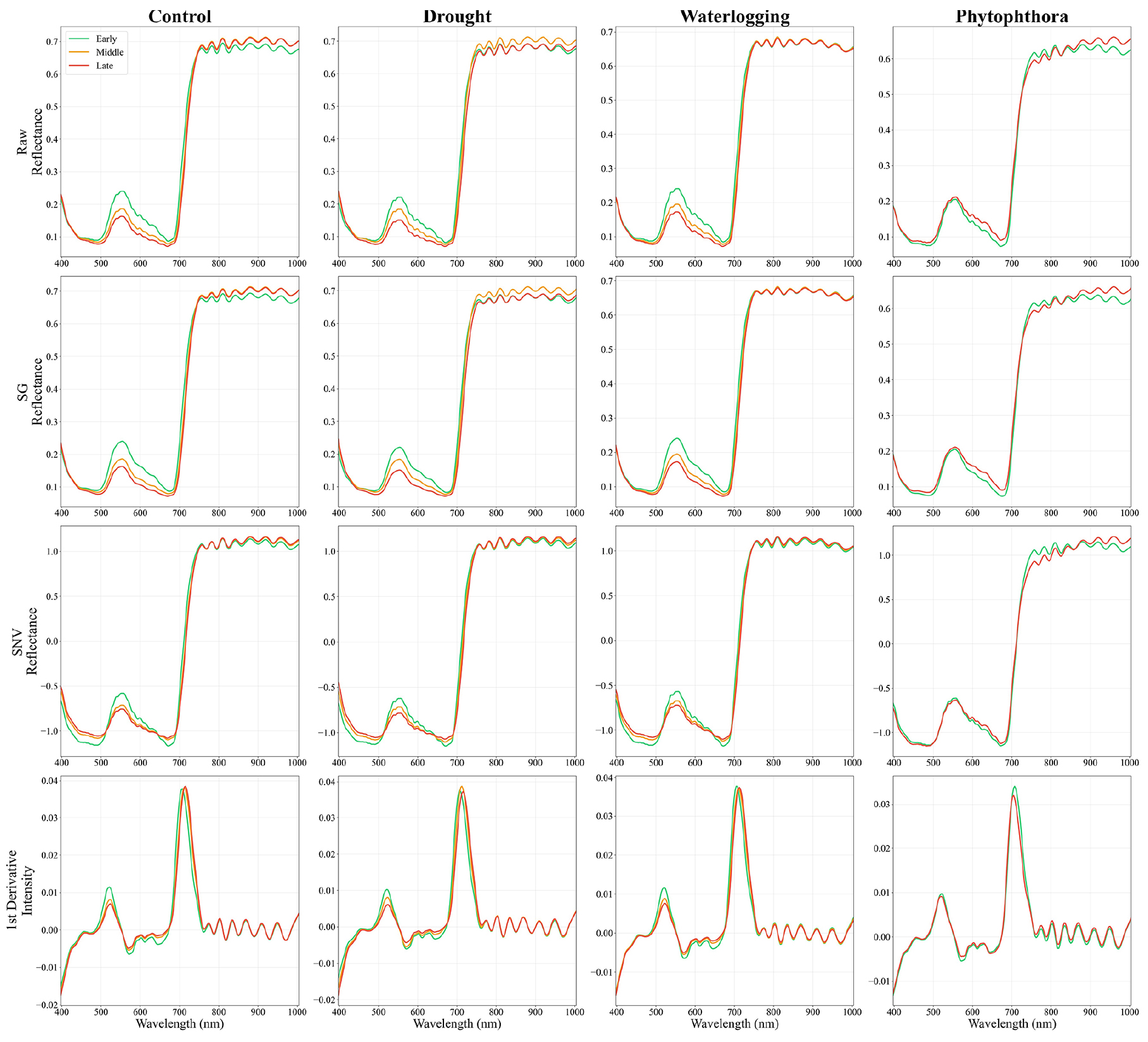
In samples from the control, drought, and waterlogging treatment groups, reflectance in the 500–600 nm range tended to decrease over time, whereas no notable changes were observed in the Phytophthora treatment group. This suggests that pathogen infection induced spectral changes distinct from those caused by environmental stress. In the near-infrared region beyond 750 nm, temporal differences in reflectance were observed in all treatment groups except the waterlogging group. However, temporal changes in reflectance were also observed in the control group, and the patterns of change in the drought and waterlogging treatment groups showed trends similar to those of the control. This indicates that the observed spectral shifts reflect a combination of changes associated with normal growth and those induced by stress, making it difficult to clearly distinguish treatment-specific spectral differences based solely on a comparison of mean spectra.

Analysis of changes in spectral characteristics according to preprocessing methods revealed that SNV preprocessing highlighted temporal variations in the 400－500 nm range, while SNV and the 1st derivative exhibited multiple peaks in the 600－700 nm range, rendering them advantageous for capturing subtle changes in the chlorophyll absorption boundary region (Smith et al., 2004). Thus, spectral differences between treatments, which appear similar in the raw spectral data, can be distinguished through appropriate preprocessing, indicating that supervised and unsupervised learning-based classification models are necessary for identification of treatment effects.

PCA by Treatment Group

PCA was performed to identify differences in spectral patterns among treatment groups based on pretreatment methods and duration of stress exposure (Fig. 4). Analysis of the cumulative explanatory power of PC1 and PC2 revealed that, for the Raw and SG preprocessing methods, PC1 exhibited high explanatory power of approximately 75% in the early stage, whereas SNV and the 1st derivative showed values ranging from 30% to 55%. While the Raw and SG preserve overall variation of the original spectrum, the spectrum information may have been reconstructed during the scattering correction process for SNV and during the gradient transformation process for the 1st derivative, resulting in the variance being distributed across multiple principal components.

As time elapsed, the explanatory power of PC1 for Raw and SG decreased to approximately 50%, suggesting that spectral variations among treatment groups diversified as stress progressed. In the early stage, the clusters of the four treatment groups were not clearly separated indicating minimal spectral differences between the treatment groups during the initial stage of stress. At the middle stage, the Phytophthora treatment group showed separation from the other treatment groups in terms of SNV and first-order derivatives; in particular, the Phytophthora group was clearly distinguished from the control and drought groups. While the clusters for the control and the drought treatment groups remained close in this stage, some overlap in the clusters for the Phytophthora and waterlogging treatment groups was observed, illustrating the difficulty in distinguishing between treatment groups using unsupervised learning alone.

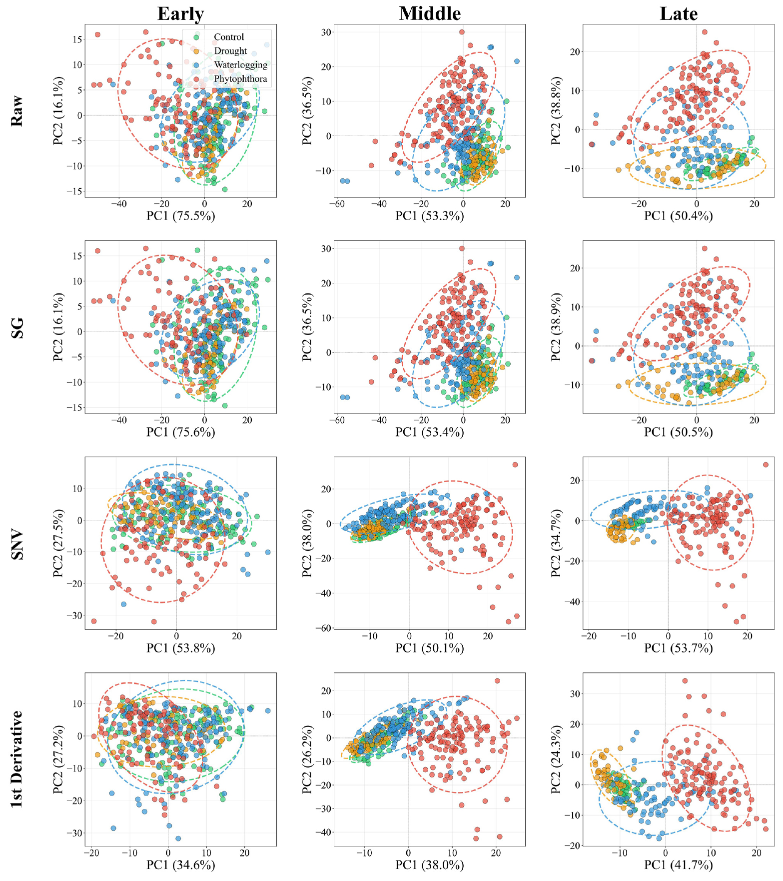
Fig. 4.

Principal component analysis (PCA) score plots of pixel-level spectral data under four treatments across three stages of stress progression (early, middle, and late) using four preprocessing methods (Raw, SG, SNV, and 1st derivative). The values in parentheses on each axis indicate the explained variance ratio (%) for PC1 and PC2.

Comparison of Classification Model Performance

The PLS-DA and 1D-CNN classification models were constructed for each stage and preprocessing method to evaluate their multi-class classification performance (Table 1).

For the PLS-DA model, the difference in F1-score between preprocessing methods was within 0.1 across all stages, indicating no significant difference in performance according to preprocessing method. In the early stage, SG preprocessing achieved the highest F1-score of 0.531, whereas in the middle and late stages, SNV preprocessing demonstrated the highest performance with scores of 0.652 and 0.688, respectively. Because PLS-DA is a model that establishes linear classification boundaries through latent variables, it is considered that the effect of spectral transformations resulting from preprocessing on these linear classification boundaries is limited (Rozenstein et al., 2014).

The 1D-CNN model showed significant performance differences depending on the preprocessing method. The 1st derivative preprocessing method demonstrated the highest performance across all stages, with an F1-score of 0.527 in the early stage, 0.772 in the middle stage, and 0.827 in the late stage. Especially, at the middle stage, the difference in F1-score between the 1st derivative (0.772) and SG (0.732) was 0.040, which is more than four times larger than the maximum difference of 0.010 observed among PLS-DA preprocessing methods during the same stage. These results suggest that the 1st derivative emphasized changes in spectral slope, highlighting subtle spectral differences between treatment groups, and the convolutional operations of the 1D-CNN effectively learns these local patterns (Ding et al., 2022; Lee et al., 2026). Although the F1 score for the 1D-CNN was the lowest, at 0.502, during the early stage, it reached 0.803 during the late stage, showing the largest performance improvement over time (0.301) among the preprocessing methods. Therefore, in the later stage of stress, when the process had progressed sufficiently, spectral differences between treatment groups became evident in the original reflectance spectrum without the need for additional spectral transformation.

The performance gap between models widened over the treatment period: in the early stage, the highest F1-score for the PLS-DA model and the 1D-CNN model was nearly identical (0.531 vs. 0.527, respectively). However, a gap of 0.120 was observed between the two models in the middle stage and this gap widened to 0.139 in the late stage. The similarity in performance of the two models in the early stage was likely due to the minimal spectral differences between treatment groups at the onset of stress, which prevented the full realization of nonlinear learning advantages. This observation is consistent with the cluster overlap in the PCA at the early stage regardless of the preprocessing method. However, the F1-score of 0.527 even in the early stage indicates that spectral differences between treatment groups partially existed in the asymptomatic stage—undetectable to the naked eye—and that the model was capable of utilizing these differences. As the spectral differences between treatment groups increased, the 1D-CNN model effectively learned the nonlinear spectral patterns that were difficult to capture using PLS-DA linear discrimination. In particular, the distinction between the waterlogging and Phytophthora-treated plots, which was difficult to achieve using unsupervised learning alone via PCA analysis, improved through 1D-CNN-based supervised learning. The multi-layer convolutional structure of the 1D-CNN effectively captured the subtle spectral differences between these two treatment groups.

Due to the limited number of samples per treatment group in this study, it was difficult to construct a diagnostic model based on individual-level learning. Therefore, multi-class classification was performed using one-dimensional spectral data at the pixel level. While the leaf area within each class differed, leading to class imbalance in the training data, at the individual level the number of plants per treatment was consistent at 25, hence the imbalance in number of pixels was due to a reduction in leaf area due to stress. In preliminary experiments, the application of inverse frequency weighting tended to increase misclassifications into minority classes. Because artificial adjustments could distort the actual spectral distribution, the original data distribution was retained, and no separate weighting was applied. Should a substantial volume of sample data be acquired in future studies to construct deep learning models at the individual level and implementing modeling that integrates spatial information, further enhancements in classification performance are anticipated.

Contribution Analysis of Classification Models

Saliency maps, generated to analyze the wavelengths contributing most significantly to classification by the best-performing 1D-CNN model in each stage, demonstrated that the chlorophyll absorption peak region of 660－690 nm contributed most to classification across all stages (Fig. 5). This wavelength band is the most sensitive to changes in chlorophyll content, suggesting that stress-induced chlorophyll degradation was a major contributor to the differences observed among treatment groups (Gitelson et al., 2003). In the early stage, the disease-treated group exhibited significantly higher saliency at 660－690 nm compared to the other treatment groups, confirming that chlorophyll-related spectral changes are present even during the asymptomatic stage when no visual manifestations are apparent. This is consistent with previous findings reporting that changes in reflectance around 695－725 nm represent the most consistent and universal response to various stressors (Carter and Knapp, 2001). As stress progressed, the model’s contributing wavelength bands expanded to the chlorophyll－carotenoid absorption region (600－640 nm) and the red-edge transition region (700－730 nm), indicating that changes in cellular structure, as well as chlorophyll degradation, were reflected in the classification (Gitelson et al., 2003). In particular, in the late stage, the saliency of the drought and waterlogging treatment groups increased significantly in the 900－950 nm water absorption region. This region corresponds to the leaf water content-sensitive wavelength band used in the water band index, indicating that water-related spectral information contributed to the classification of the water-stress treatment groups (Peñuelas et al., 1997). In contrast, the Phytophthora-affected plot showed a high contribution in the red-edge transition region (700－730 nm), confirming that classification was based on wavelength information distinct from that associated with water stress. The difference in the contributing wavelength bands across these processing channels indicates that the 1D-CNN learned the unique spectral patterns of each channel rather than simply the average difference across the entire spectrum. This finding contrasts with the observation that classification based solely on a visual comparison of the raw spectra proved unattainable.

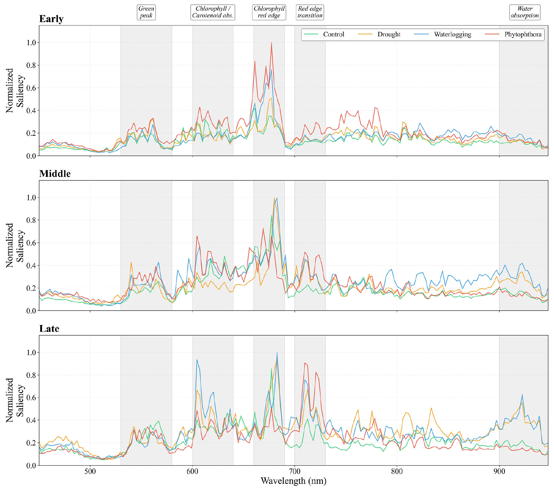
Fig. 5.

Saliency maps of the one-dimensional convolutional neural network (1D-CNN) model with 1st derivative preprocessing, showing wavelength-specific contributions to classification for each treatment across three stages of stress progression: early, middle, and late. Shaded regions indicate physiologically relevant spectral bands—the green peak at 530－580 nm, chlorophyll, and carotenoid absorption at 600－640 nm, the chlorophyll red edge at 660－690 nm, the red edge transition at 700－730 nm, and water absorption at 900－950 nm. Saliency values were normalized to the maximum value within each stage.

Pixel-Level Classification Map Visualization

Pixel-level classification maps of hyperspectral images were generated by applying the optimal 1D-CNN model for each stage (Fig. 6). The control group was classified reasonably accurately at each of the three stages. In contrast the drought group was classified into a mix of several classes during the early stage; however, classification accuracy improved as the experiment progressed to the late stage. Even in the late stage, some pixels from the drought group were misclassified as belonging to the control group, consistent with overlap of the clusters for these two treatment groups in the PCA analysis. Misclassification was most frequent between the waterlogging and Phytophthora treatment plots, resulting from the similar spectral characteristics induced by the two treatments. Especially, pixels corresponding to leaf veins in the control group tended to be misclassified as wet; leaf veins have a higher water content than leaf tissue and thus exhibit spectral characteristics similar to those of the water stressed group.

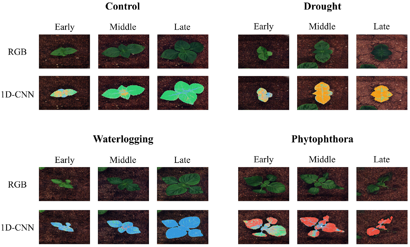
Fig. 6.

Pixel-level classification maps generated by the best one-dimensional convolutional neural network (1D-CNN) model (with 1st derivative preprocessing) for each stage of stress progression. Each column represents a treatment (control, drought, waterlogging, and Phytophthora), and each row represents a stage (early, middle, and late). Colors indicate predicted classes: green (control), yellow (drought), blue (waterlogging), and red (Phytophthora).

Limitations and Future Perspectives

This study has several limitations. First, this study was conducted using a single perilla cultivar, 'Anyu,' and future studies incorporating multiple cultivars are expected to strengthen the generalizability of the classification model by accounting for inter-cultivar differences in spectral characteristics. Second, although the experiment was conducted under controlled growth chamber conditions, the hyperspectral imaging-based classification technique is expected to be applicable to field environments through standardization of sensor calibration and imaging protocols. Third, as noted above, the limited number of samples per treatment necessitated pixel-level classification, which resulted in class imbalance due to differences in leaf area among treatments. Future studies incorporating multiple cultivars and large-scale field experiments are needed to validate the generalizability of the model. Additionally, the application of individual-level learning and multidimensional modeling that integrates spatial information is expected to further improve classification performance.