

Introduction
Materials and Methods
Image acquisition
Radiometric calibration
Extraction of meeting ground between each image
Statistical Analysis
Results and Discussion
Introduction
In order to evaluate crop status in the field, a large amount and various types of information are required. Traditional crop evaluation method in the field is manually taking samples of crops, resulting in destructive, time-consuming, and laborious. However, remote sensing technique can acquire crop data with non-destructive and non-laborious methods rapidly (Lillesand et al., 2015). With the development of high performing sensors and platforms, remote sensing become a promising technique. Among remote sensing platforms, aerial platforms including satellite, manned aircraft and unmanned aerial vehicle (UAV) can provide a high-throughput data acquisition in field detection. Recently, remote sensing using UAV platform has been studied a lot due to the advantages of UAV platform which provide high spatial and temporal resolution inexpensively compared to satellite and manned aircraft (Muchiri and Kimathi, 2016; Shi et al., 2016).
However, the complexity of Earth’s components such as the land and atmosphere and condition of illumination can affect data acquisition with various errors such as atmospheric effect, geometric error and radiometric error (Shahtahmassebi et al., 2013). Especially, shadows are major sources causing radiometric problem in the field with false color tone of vegetation. Moreover, shadows reduce the success of image processing for extraction of crop information, interrupting feature extraction, image matching, and change detection (Junli and Shugen, 2002; Singh et al., 2012). Thus, the adverse effect of shadows is required to be analyzed for the generation of high-quality image data. However, there is a little research in remote sensing using the UAV platform despite of active study in using satellite (Yamazaki et al., 2009; Liu and Yamazaki, 2012; Singh et al., 2012; Milas et al., 2017). In the current paper, the effects of shadow in RGB images using the UAV platform are reported to improve image data remotely sensed by the UAV platform so that researchers can be aware of this issue.
Materials and Methods
Image acquisition
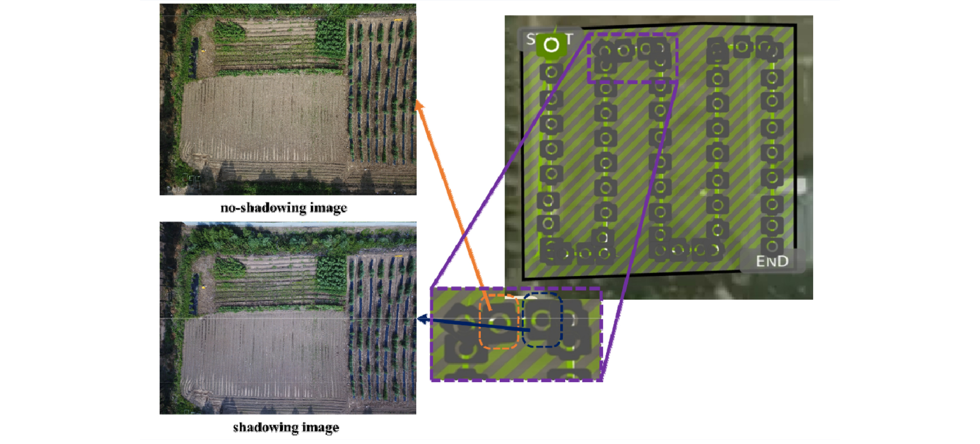
The shadowing image and no-shadowing image by cloud were acquired using an RGB camera mounted on the UAV platform (Mavic 2 Zoom, DJI, China) on 26 July 2019 (Table 1). The images were captured on the waypoint path automatically set by Pix4Dcapture (Pix4D SA, Lausanne, Switzerland), UAV flight planning application. The shadowing image was capture immediately after the no-shadowing image (Fig. 1). The test field is located at Jeju National University (33°72'N, 126°33'E, altitude 257 m), 102, Jejudaehak-ro, Jeju-si, Jeju-do, Republic of Korea.
Table 1. Specification of the RGB camera mounted on the UAV platform (Mavic 2 Zoom) used in the study
| Item | Specification |
| Resolution | 4000 × 3000 |
| Image sensor | 1/2.3" CMOS |
| Focal length | 24‒48 mm |
| Field of view | 72.3° (horizontal), 57.5° (vertical) |
| F-stop (aperture) | 2.8‒3.8 |
| Shutter speed | 8‒1/8000 s |
Radiometric calibration
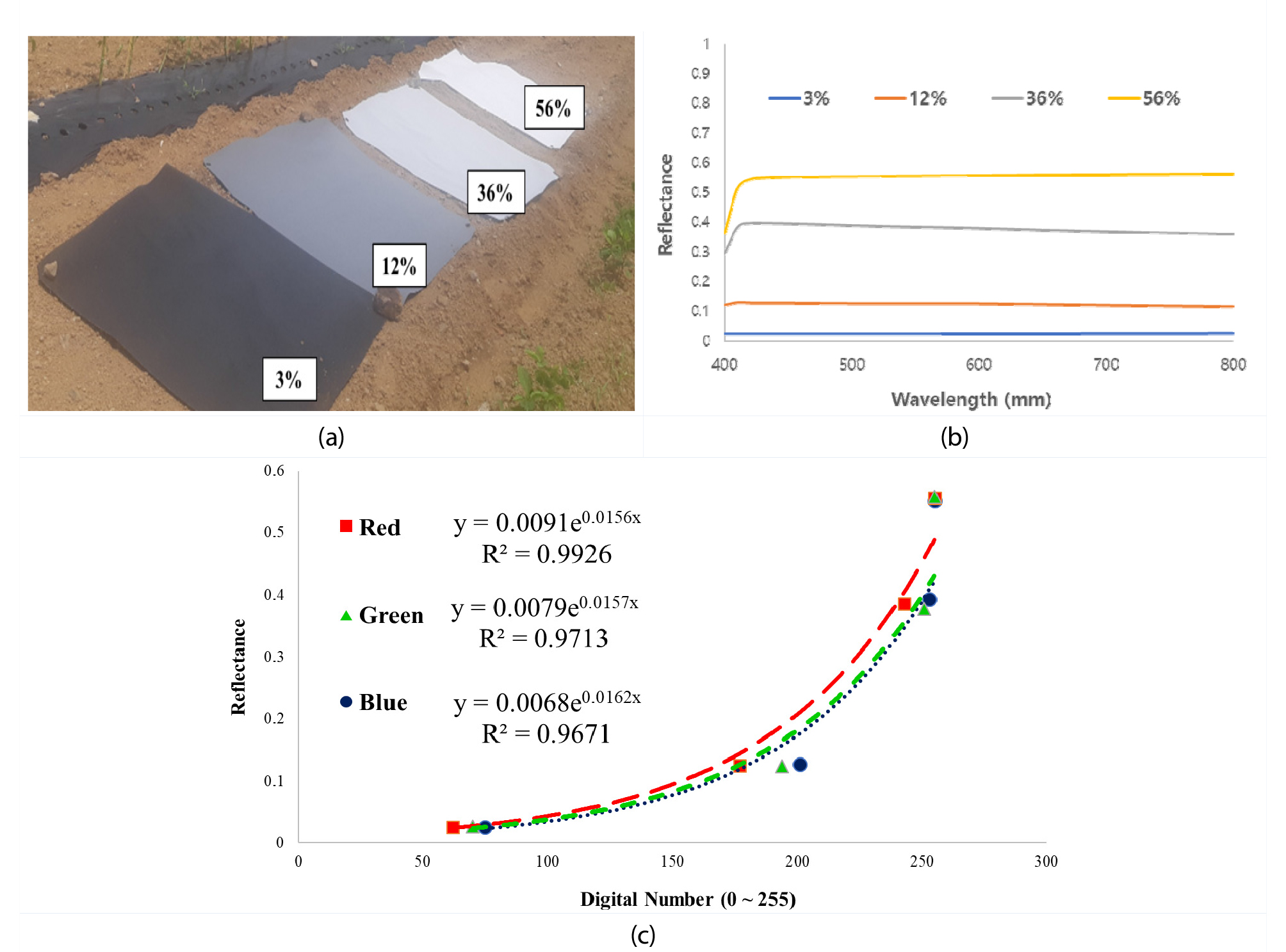
The conditions of illumination and atmosphere are ever-changing, resulting in the radiometric errors of the image captured by an RGB camera. Thus, the digital number (DN) of the RGB camera should convert to the standard reflectance. In this study, the empirical line method was used for radiometric calibration (Smith and Milton, 1999). Calibration targets (1.2 by 1.2 m Group 8 Technology Type 822 ground calibration panels), which provide the standard reflectance value with four scales (3%, 12%, 36%, and 56%) were placed in the test field (Fig. 2A). The DNs of each red, green, and blue band were extracted from the image, including the calibration target by ArcGis 10.6 (ESRI, Redlands, USA), geographic information system software. The extracted DNs were fitted to the reflectance value, generating equation (1). On 26 July 2019, the generated exponential regression model in each band was shown in (Fig. 2C). Finally, the equation was applied to the DNs in both shadowing image and no-shadowing image converting to the standard reflectance value.
| $$r_k=A_ke^{B_kDN}$$ | (1) |
Extraction of meeting ground between each image
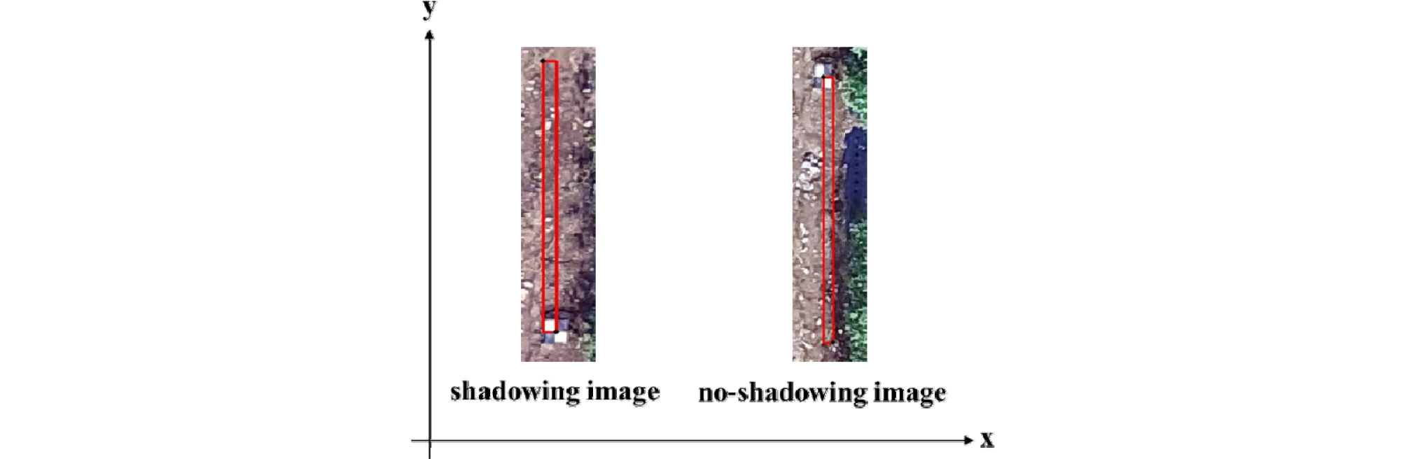
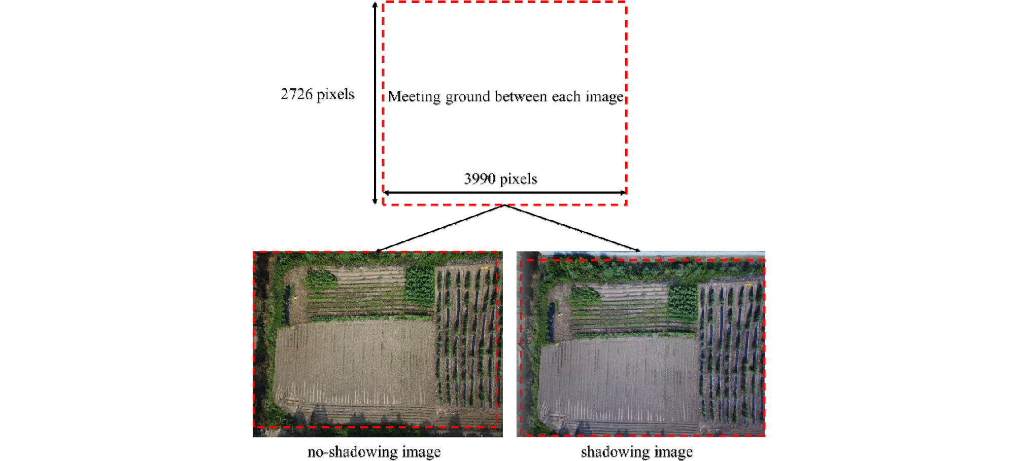
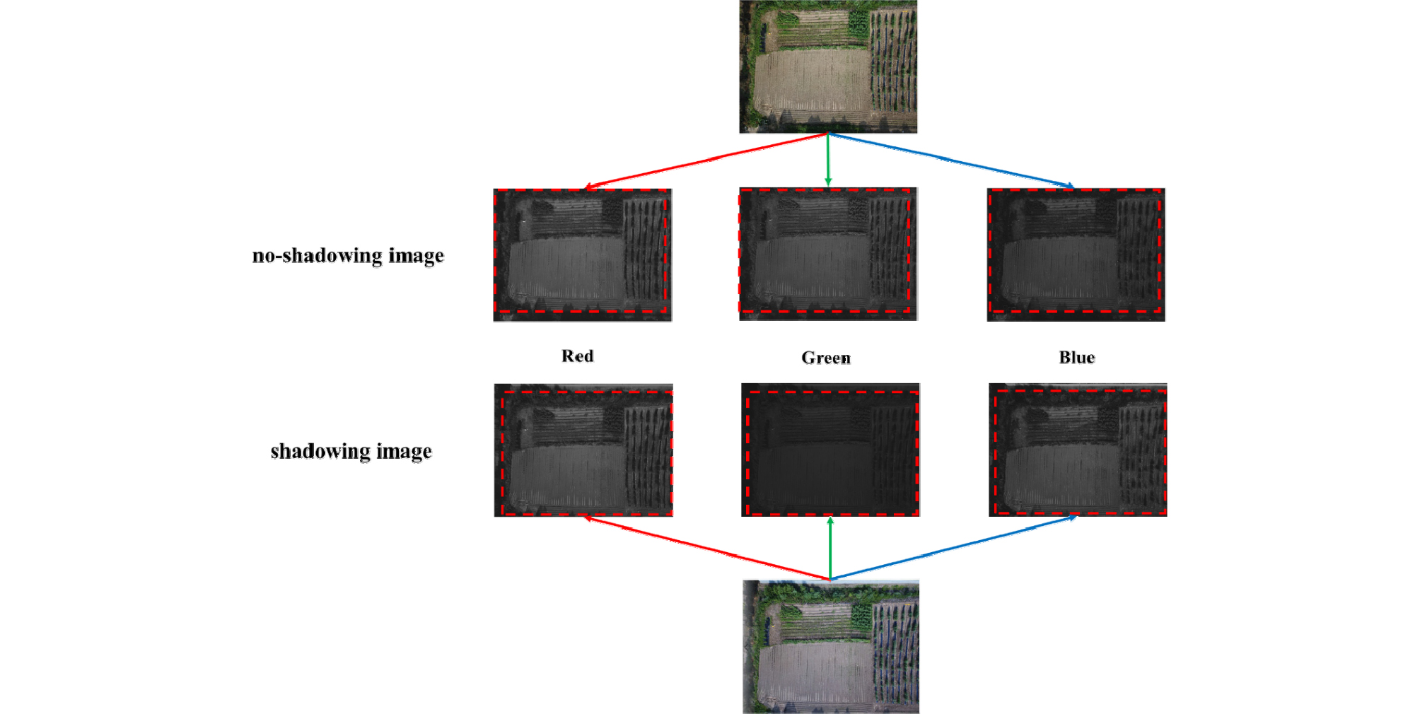
Shadowing image and no-shadowing were captured at different sites on the straight travel of the UAV platform (Fig. 3). Thus, the meeting ground between each image was extracted by the calculation of the differences of the x-axis and y-axis distance. In each image, white and black panel providing the position indicatable by 1 pixel on its center was appeared in common (Fig. 3). Based on the position of white and black panel’s center, the differences of the x-axis and y-axis distance were calculated to 10 pixels and 274 pixels respectively. That means the shadowing image was captured at the position in the x-axis direction, -10 pixels and in the y-axis direction, 274 pixels from the no-shadowing image. As a result, the meeting ground was extracted as 3990 pixels in the x-axis and 2726 pixels in the y-axis (Fig. 4) within each image.
Statistical Analysis
In the current study, the shadow image was compared to the on-shadowing image (Fig. 5). Statistical analysis consisted of fitting Bayesian linear regression to verify the association between the presence or absence of the shadows and the color channels (red, green, and blue). The statistical model follows:
| $$y_i=\beta_0+\beta_1x_i+\epsilon_i$$ | (2) |
where, is the intercept, is the slope of straight line, .
Vague priors are assumed for regression coefficients and error variance.
| $$\beta_j\sim N(0,\tau_j^2),11j=1,2$$ | (3) |
where, and
| $$\frac1{\sigma^2}\sim\Gamma(\frac{c_0}2,\frac{d_0}2)$$ | (4) |
where, .
Significance of the shadows effects was tested using the Bayes factor. In an overview, the Bayes factor measure which model is more plausible given the data (Gelman et al., 2014).
| $$B_{12}=\frac{p(y\left|M_1)\right.}{p(y\left|M_2)\right.}\;\Rightarrow\log B_{12}=\log pp(y\left|M_1)-\log pp(y\left|M_2)\right.\right.$$ | (5) |
where, is the Bayes factor, are models 1 and 2, respectively. All computations were done using R statistical software (R Core Team, 2018) and MCMCpack R package (Martin et al., 2011).
Results and Discussion
Box plots of the distribution of RGB values suggest that shadow effects are significant for colors blue and green, but for red color the difference between the two groups is not quite high (Fig. 6). However, Bayes factor results reveal that models with shadow effects included in the linear predictor is more likelihood, i.e, the shadows effect is significant for all channel colors (Table 2). Interestingly, the shadow effect is less for red color, unlike green and blue. This could be because the compared images were soil, which contains red color more than others. It might have different results if vegetative images were compared. It could be worth to compare only between vegetative areas to determine shadow effects.
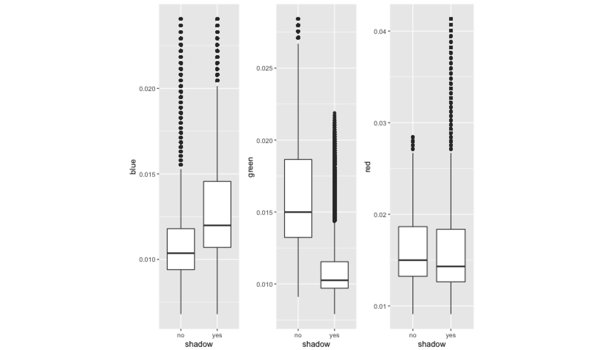
Table 2. Posterior means of the shadow effect and standard deviation from the posterior distribution of the shadow effects, and the natural logarithm Bayes Factor
| Models | Shadow effect | Standard deviation | log Bayes Factor |
| Blue | 0.0023 | <0.0001 | 79671 |
| Green | -0.0056 | <0.0001 | 319730 |
| Red | 0.0001 | <0.0001 | 55.8 |
The current study examined the shadow effects in the image analysis captured from UAV. Considering the current research trend using UAV, this issue is very important to know to perform experiments properly. Thus, we report this result with excitement to help researchers who do field experiments with UAV derived image analysis.
